Chinese Physics Letters, 2022, Vol. 39, No. 2, Article code 027401 Superconductivity with a Violation of Pauli Limit and Evidences for Multigap in $\eta$-Carbide Type Ti$_4$Ir$_2$O Bin-Bin Ruan (阮彬彬)1,2*, Meng-Hu Zhou (周孟虎)1,2, Qing-Song Yang (杨清松)2,3, Ya-Dong Gu (谷亚东)2,3, Ming-Wei Ma (马明伟)2, Gen-Fu Chen (陈根富)2,3, and Zhi-An Ren (任治安)2,3* Affiliations 1Songshan Lake Materials Laboratory, Dongguan 523808, China 2Institute of Physics and Beijing National Laboratory for Condensed Matter Physics, Chinese Academy of Sciences, Beijing 100190, China 3School of Physical Sciences, University of Chinese Academy of Sciences, Beijing 100049, China Received 14 December 2021; accepted 12 January 2022; published online 29 January 2022 *Corresponding author. Email: bbruan@mail.ustc.edu.cn; renzhian@iphy.ac.cn Citation Text: Ruan B B, Zhou M H, Yang Q S et al. 2022 Chin. Phys. Lett. 39 027401    Abstract We report the synthesis, crystal structure, and superconductivity of Ti$_4$Ir$_2$O. The title compound crystallizes in an $\eta$-carbide type structure of the space group $Fd\bar{3}m$ (No. 227), with lattice parameters $a=b=c=11.6194(1)$ Å. The superconducting temperature $T_{\rm c}$ is found to be 5.1–5.7 K. Most surprisingly, Ti$_4$Ir$_2$O hosts an upper critical field of 16.45 T, which is far beyond the Pauli paramagnetic limit. Strong coupled superconductivity with evidences for multigap is revealed by the measurements of heat capacity and upper critical field. First-principles calculations suggest that the density of states near the Fermi level originates from the hybridization of Ti-3$d$ and Ir-5$d$ orbitals, and the effect of spin-orbit coupling on the Fermi surfaces is prominent. Large values of the Wilson ratio ($R_{\rm W} \sim 3.9$), the Kadowaki–Woods ratio [$A/\gamma^2 \sim 9.0 \times 10^{-6}$ $µ\Omega\cdot$cm/(mJ$\cdot$mol$^{-1}\cdot$K$^{-1}$)$^2$], and the Sommerfeld coefficient ($\gamma = 33.74$ mJ$\cdot$mol$^{-1}\cdot$K$^{-2}$) all suggest strong electron correlations (similar to heavy fermion systems) in Ti$_4$Ir$_2$O. The violation of Pauli limit is possibly due to a combination of strong-coupled superconductivity and large spin-orbit scattering. With these intriguing behaviors, Ti$_4$Ir$_2$O serves as a candidate for unconventional superconductor.
cpl-39-2-027401-fig1.png
cpl-39-2-027401-fig2.png
cpl-39-2-027401-fig3.png
cpl-39-2-027401-fig4.png
DOI:10.1088/0256-307X/39/2/027401 © 2022 Chinese Physics Society Article Text For their superior abilities to carry large currents, superconductors have been widely used to generate high magnetic fields at different settings, such as medical magnetic resonance imaging (MRI), maglevs, and particle accelerators.[1,2] However, applications to these uses have been limited to only a few superconducting compounds, primarily NbTi or Nb$_3$Sn.[3] Apart from the superconducting transition temperature ($T_{\rm c}$), the critical current density, and the ductibility, one major limitation comes from the upper critical field ($H_{\rm c2}$) in a type-II superconductor. At low temperatures, the Zeeman energy splitting ($\Delta E$) is the key factor limiting $H_{\rm c2}$. When the external magnetic field is large enough ($\ge \mu_0H_{\rm P}$), driving $\Delta E$ comparable with twice the superconducting energy gap, the Cooper pairs are broken. In a Bardeen–Cooper–Schrieffer (BCS) weak coupling scenario, the Pauli paramagnetic limit (or, Pauli limit for short) is expressed by $\mu_0H_{\rm P} = 1.86 \times T_{\rm c}$ (T/K). $H_{\rm c2}$ of most type-II superconductors falls below $H_{\rm P}$, regardless of the value of $T_{\rm c}$.[4] However, a violation of the Pauli limit is often regarded as a side evidence for unconventional superconductivity, as in heavy fermions,[5] iron-based superconductors,[6] non-centrosymmetric superconductors,[7,8] and more recently, in $A_2$Cr$_3$As$_3$ ($A$ = Na, K, Rb, Cs)[9–11] or magic-angle twisted trilayer graphene.[12] In addition to unconventional superconductivity, large spin-orbit scattering,[13] strong electron-phonon coupling,[14] or a highly anisotropic structure[15] all tend to increase $H_{\rm c2}$, pushing it beyond $H_{\rm P}$. Nevertheless, superconductors with a violation of Pauli limit are still very rare. In this study, we focus on a suboxide of the so-called $\eta$-carbide family, also known as the E9$_3$-type phases. The $\eta$-carbide type phase adopts a cubic crystal structure of the space group $Fd\bar{3}m$ (No. 227), which is derived from the Ti$_2$Ni type after small atoms, typically C, N, or O, take the interstitial sites. W$_3$Fe$_3$C, the first member in the family, was discovered in the 1950s.[16,17] Since then, a large number of carbides, nitrides, and oxides of the same structural family have been reported. Depending on different crystallographic sites the atoms take, there are four stoichiometries of $\eta$-carbide type phases, namely (T and T$'$ stand for transition metals, $X$ = C, N, O): (a) T$_4$T$'_2X$, as in Mo$_4$Co$_2$C, Zr$_4$Re$_2$O;[17](b) T$_3$T$'_3X$, as in W$_3$Fe$_3$C, Nb$_3$Cr$_3$N;[16](c) T$_6$T$'_6X$, as in Mo$_6$Ni$_6$C;[18] (d) T$_8$T$'_4X$, as in Nb$_8$Zn$_4$C.[19] Although they have been discovered for more than half a century, reports on these phases mainly focus on their hardness,[20] the hydrogen-sorption,[21] or the catalytic abilities,[22] few of them have been examined for their electronic properties. Ku et al. reported several $\eta$-carbide type superconductors in 1984,[23] including Ti$_4$Co$_2$O ($T_{\rm c} = 3.1$ K), Zr$_4$Os$_2$O ($T_{\rm c} = 3.0$ K), Nb$_4$Rh$_2$C ($T_{\rm c} = 8.9$ K), etc. Recently, superconductivity in Zr$_4$Rh$_2$O$_{0.6}$[24] and Nb$_4$Rh$_2$C$_{1-\delta}$[25] was systematically studied. Nb$_4$Rh$_2$C$_{1-\delta}$ was found to host a large $\mu_0H_{\rm c2}(0)$ of 28.5 T, violating the Pauli paramagnetic limit. This is not trivial since $\eta$-carbide type phases are not highly anisotropic in their crystal structures. Thus, strong electron correlations, or even unconventional superconductivity, can be expected in the superconductors of $\eta$-carbide type. However, evidences for these speculations are still absent. In this Letter, we report the synthesis and a systematical study of superconductivity in Ti$_4$Ir$_2$O. Bulk superconductivity of $T_{\rm c} = 5.12$ K is revealed by magnetic susceptibility and heat capacity measurements, confirming a previous report by Matthias et al. in 1963.[26] In that paper, superconductivity in “Ti$_{0.573}$Ir$_{0.287}$O$_{0.14}$” was reported without further details. Notice that such an early study needs reexamination. For example, superconductivity of $T_{\rm c} = 11.8$ K in “Zr$_{0.61}$Rh$_{0.285}$O$_{0.105}$” reported in the same paper[26] was later ascribed to CuAl$_2$-type Zr$_2$Rh.[27] In addition, superconducting parameters of Ti$_4$Ir$_2$O are determined in our study, among which the $\mu_0H_{\rm c2}(0)$ is 16.45 T, far above the Pauli limit (9.52 T). Moreover, the deviation of $\mu_0H_{\rm c2}(T)$ from the Werthamer–Helfand–Hohenberg (WHH) theory, and the heat capacity in the superconducting state suggest a multigap nature. Large electron correlations in Ti$_4$Ir$_2$O are evidenced by both experimental results and first-principles calculations. Methods. Polycrystalline samples of Ti$_4$Ir$_2$O were prepared by solid state reactions. Stoichiometric amount of titanium (powder, 99.99%), iridium (powder, 99.99%), and TiO$_2$ (powder, 99.95%) was mixed thoroughly, and then cold pressed into pellets. The pellets were placed in corundum crucibles, which were subsequently sealed into niobium tubes under purified argon. The niobium tubes were heated to 1800 K, held at the temperature for 20 hours, and then cooled down to room temperature by switching off the furnace. To avoid the oxidation of niobium tubes at high temperatures, heating treatments were carried out under an argon atmosphere. Grey and dense solid was obtained after opening the niobium tubes. No reaction between the samples and the niobium tubes was observed, and the weight losses after the reactions were negligible. We also performed reactions at lower temperatures or using arc-melting methods. However, these alternative methods did not produce single-phase samples (see the Supplementary Material). Powder x-ray diffraction (XRD) measurements were carried out on a PAN-analytical x-ray diffractometer equipped with Cu $K_\alpha$ radiation at room temperature. The Rietveld refinement of the XRD results was performed with the Gsas package.[28] Temperature-dependent electrical resistivity and heat capacity of the sample were measured on a Quantum Design physical property measurement system (PPMS). DC magnetization was measured on a Quantum Design magnetic property measurement system (MPMS). Details for the physical property measurements can be found elsewhere.[29] All the data from the magnetization measurements were corrected based on the demagnetization factor, which was determined by the dimensions of the rectangular sample.[30] First-principles calculations were carried out in the frame of the density functional theory (DFT), using the Quantum espresso (QE) package.[31–33] Generalized gradient approximation (GGA) exchange-correlation functionals of PBEsol[34] were selected, together with the projector augmented wave pseudopotentials from the PSlibrary package.[35] To take spin-orbit coupling (SOC) into account, we performed both the scalar-relativistic and fully relativistic calculations. Energy cutoffs were 100 Ry and 1000 Ry for the wavefunctions and the charge densities, respectively. A Monkhorst–Pack grid of $8^{3}$ $k$-points was used for the self-consistent calculation, and a denser grid of $12^{3}$ $k$-points was used to generate the density of states (DOS). Before the self-consistent calculation, the cell parameters, as well as the atomic positions, were fully relaxed starting from the experimental values, using the Broyden–Fletcher–Goldfarb–Shanno (BFGS) algorithm. The grid of $k$-mesh was checked for convergence. The Barder analysis was performed with the help of the Critic2 package.[36] Fermi surfaces were constructed on a superfine grid of $101^{3}$ $k$-points, with the help of maximally localized Wannier functions (MLWFs) generated by the Wannier90 code.[37,38] Results. Figure 1 displays the powder XRD pattern of Ti$_4$Ir$_2$O collected at room temperature. We find that Ti$_4$Ir$_2$O crystallizes in an $\eta$-carbide type structure, which is of the space group $Fd\bar{3}m$ (No. 227). In the structure, Ti and Ir form a Ti$_2$Ni-type framework, where O takes the 16$c$ (distorted octahedral) interstitial sites (see the inset of Fig. 1). We note that the inclusion of oxygen is key to stabilize the Ti$_4$Ir$_2$O phase, since no Ti$_2$Ni-type Ti$_2$Ir phase can be acquired (nor has it been reported in the Ti–Ir phase diagram[39]). The crucial roles of interstitial C, N, or O have been frequently observed in other $\eta$-carbide type phases, such as W$_3$Fe$_3$C,[17] Zr$_4$Pd$_2$N,[23] or Zr$_4$Rh$_2$O.[24] Rietveld refinement was performed and the result is shown in Fig. 1, giving cell parameters $a=b=c=11.6194(1)$ Å. The value is close to the reference one 11.620 Å.[26] The occupancy on each site is refined to be 1.0 (except for that of oxygen, which is fixed to 1). Detailed refined crystallographic parameters are summarized in Table 1. The fully relaxed cell parameters and atomic positions are also listed for comparison. Notice that the discrepancies between the DFT values and the experimental values are within 0.6%, and the inclusion of SOC has negligible effects on the crystallographic parameters.
cpl-39-2-027401-fig1.png
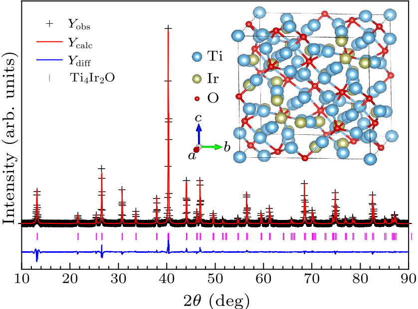
Fig. 1. Room-temperature XRD pattern of Ti$_4$Ir$_2$O and its Rietveld refinements. $Y_{\rm obs}$, $Y_{\rm calc}$, and $Y_{\rm diff}$ stand for the observed intensity, the calculated intensity, and the difference between them, respectively. The vertical bars indicate the Bragg positions for $\eta$-carbide type Ti$_4$Ir$_2$O. The conventional unit cell is shown as the inset.
Table 1. Crystallographic parameters of Ti$_4$Ir$_2$O from Rietveld refinement of room temperature XRD. Numbers in parentheses indicate the standard deviations in the last digit. Parameters from first-principles calculations are also listed for comparison. Here $R_{\rm p}=5.80\%$, $R_{\rm wp}=3.49\%$; $y_{_{\scriptstyle \rm Ti1}}=z_{_{\scriptstyle \rm Ti1}}=0$, $y_{_{\scriptstyle \rm Ti2}}=z_{_{\scriptstyle \rm Ti2}}=0.125$, $x_{_{\scriptstyle \rm Ir}}=y_{_{\scriptstyle \rm Ir}}=z_{_{\scriptstyle \rm Ir}}$, $x_{_{\scriptstyle \rm O}}=y_{_{\scriptstyle \rm O}}=z_{_{\scriptstyle \rm O}}$; $U_{\rm eq}$ is defined as one-third of trace of the orthogonalized $U_{ij}$ tensor.
Space group $Fd\bar{3}m$ (No. 227)
$a$ (Å) 11.6194(1)
$a_{_{\scriptstyle \rm w/o-SOC}}$ (Å) 11.5562
$a_{_{\scriptstyle \rm with-SOC}}$ (Å) 11.5531
Atom (position)   $x$ $U_{\rm eq}$ (0.01 Å$^2$)  $x_{_{\scriptstyle \rm w/o-SOC}}$  $x_{_{\scriptstyle \rm with-SOC}}$
Ti1 (16$c$) 0 0.348(60) 0 0
Ti2 (48$f$) 0.4412(2) 0.065(25) 0.4428 0.4419
Ir (32$e$) 0.2145(0) 0.276(24) 0.2160 0.2159
O (16$d$) 0.5 0.633(150) 0.5 0.5
Superconductivity is evidenced in both resistivity and magnetization measurements, as shown in Fig. 2. At the normal state, Ti$_4$Ir$_2$O displays a metallic behavior, with the resistivity ($\rho$) decreasing upon cooling. The residual resistivity ratio (RRR = $\rho$(300 K)/$\rho$(6 K) = 1.39) is quite small, which is typical for a transition metal suboxide (for example, see Refs. [24,40]). The normal state $\rho(T)$ shows a convex feature (saturation) above 50 K. This can be explained with a parallel-resistor model, in which a strong electron-phonon coupling takes place (see, for instance, the A15 superconductors[41,42] and SrPt$_3$P[43]). Alternatively, it can be interpreted by an inter-band scattering, known as the Bloch–Grüneisen–Mott (BGM) mechanism.[29,44,45] The inset in Fig. 2 shows $\rho(T)$ below 70 K. We can find that the data below 35 K follow a Fermi liquid behavior: $$ \rho(T) = \rho_0 + AT^2,~~ \tag {1} $$ giving $\rho_0 = 0.263$ m$\Omega\cdot$cm, $A = 10.25$ n$\Omega\cdot$cm$\cdot$K$^{-2}$. At lower temperatures, $\rho(T)$ starts to drop from 5.22 K ($T_{\rm c}^{\rm onset}$), reaching zero at 5.13 K ($T_{\rm c}^{\rm zero}$), indicating the occurrence of superconductivity. Such a sharp transition implies a superior homogeneity of our sample. In Fig. 2(b), we show the DC magnetic susceptibility ($\chi$) of Ti$_4$Ir$_2$O from 1.8 K to 8.0 K. The large diamagnetic signal in the zero-field cooling (ZFC) process confirms the bulk nature of the superconductivity. The field cooling (FC) gives a much smaller diamagnetism, suggesting a substantial pinning effect in the sample. $T_{\rm c}$ is determined to be 5.12 K from the first point to deviate from the normal state noises on the ZFC curve, which is in very good agreement with the value from $\rho(T)$. In the inset of Fig. 2(b), we show the temperature dependence of magnetization at the normal state, from which a Curie–Weiss behavior can be inferred.
cpl-39-2-027401-fig2.png
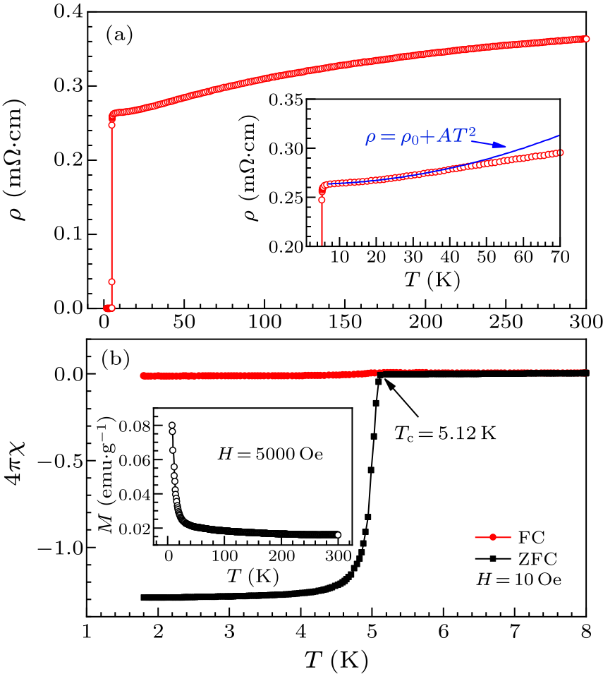
Fig. 2. (a) Temperature dependence of resistivity of Ti$_4$Ir$_2$O under zero magnetic field. Normal state data below 35 K can be described by Eq. (1), as shown in the inset. (b) Temperature dependence of DC magnetic susceptibility of Ti$_4$Ir$_2$O at low temperatures. Inset shows the temperature dependence of the normal state magnetization from 8 K to 300 K.
Figure 3(a) shows the superconducting transition under various magnetic fields. Clearly, the transition is suppressed to lower temperatures when applying external fields. However, the suppression of $T_{\rm c}$ is very slow. For instance, under a magnetic field of 9 T, $T_{\rm c}$ is still above 2.5 K. Temperature dependence of the heat capacity ($C_{\rm p}$) shows a distinct anomaly at low temperatures [Fig. 3(d)], which validates the bulk superconductivity again. $T_{\rm c}$ can be determined from the $C_{\rm p}/T$–$T$ curves based on an entropy balance method. At zero magnetic field, $T_{\rm c}$ determined from $C_{\rm p}$ is 5.12 K, which is in excellent agreement with the values from $\rho(T)$ and $\chi(T)$. Results from $\rho(T)$ and $C_{\rm p}/T$–$T$ under various magnetic fields allow us to determine $H_{\rm c2}$ of Ti$_4$Ir$_2$O. In Fig. 3(f), the points from the $\rho(T)$ measurements are determined from the midpoints of the superconducting transitions, while points from $C_{\rm p}/T$–$T$ curves are determined using the method described above, error bars correspond to the transition width. The data from $\rho(T)$ and $C_{\rm p}/T$–$T$ agree well with each other, while the transition widths are larger in the $C_{\rm p}$ measurements. The Pauli paramagnetic limit for a superconductor with $T_{\rm c} = 5.12$ K is $\sim $9.52 T. However, as shown in Fig. 3(f), superconductivity still survives when the magnetic field is 12 T. This conclusively indicates a violation of Pauli limit in Ti$_4$Ir$_2$O.
cpl-39-2-027401-fig3.png
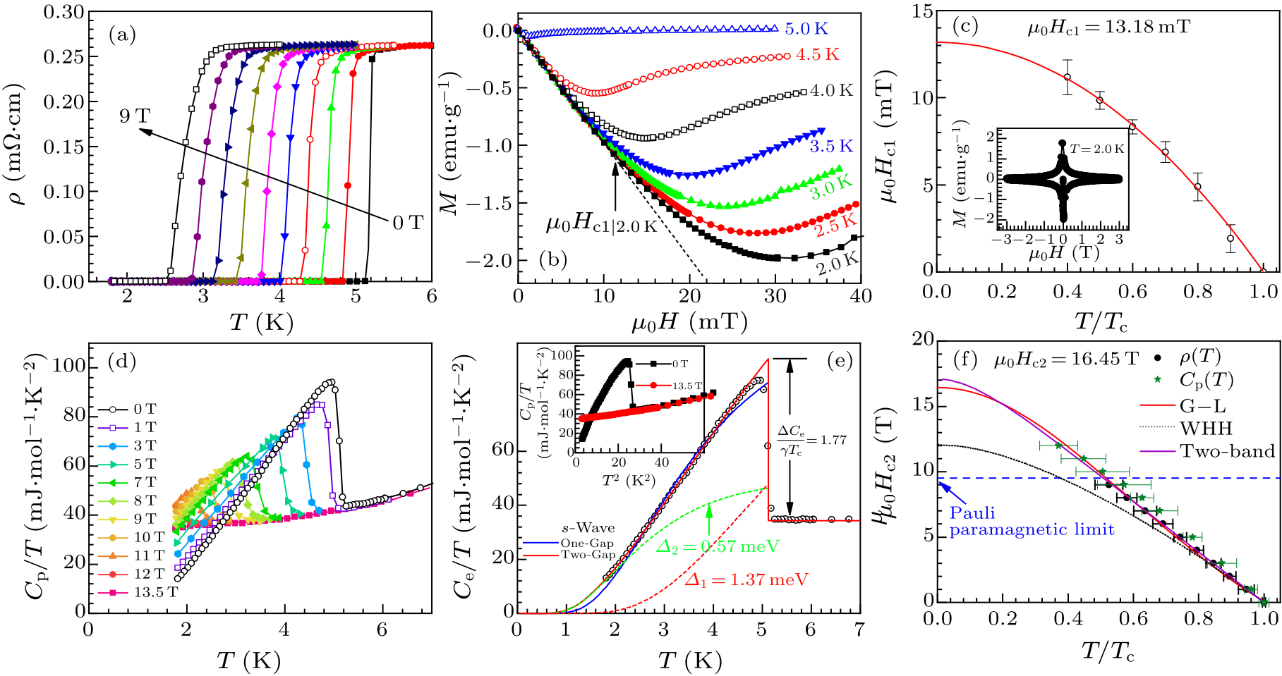
Fig. 3. (a) Superconducting transition on $\rho(T)$ under magnetic fields from 0 T to 9 T, the field increment between each curve is 1 T. (b) Isothermal magnetization under different temperatures. The dashed line shows the initial Meissner states. (c) Lower critical fields ($H_{\rm c1}$) under different temperatures, and the fit according to the G–L relation. Inset shows the isothermal magnetization loop at 2.0 K. (d) Low temperature heat capacity under magnetic fields from 0 T to 13.5 T. (e) Electronic contribution of heat capacity at zero magnetic field. Solid curves show fits based on a one-gap s-wave model (blue), and a two-gap s-wave model (red). Contributions from the two gaps are displayed as dotted curves. (f) Upper critical fields ($H_{\rm c2}$) under different temperatures, determined by $\rho(T)$ and $C_{\rm p}(T)$. The fitting curves are based on the $\rho(T)$ data, according to the G–L (red), WHH (dotted), and two-band (purple) models, respectively. The value of $\mu_0H_{\rm c2}(0)$ is from the G–L fit.
The fit to $H_{\rm c2}$ is carried out using the WHH relation:[46] $$\begin{align} \ln\Big(\frac{1}{t}\Big)={}&\Big(\frac{1}{2}+\frac{i\lambda_{_{\scriptstyle \rm SO}}}{4\gamma_{\rm w}}\Big)\psi \Big(\frac{1}{2}+\frac{h+i\gamma_{\rm w}+\lambda_{_{\scriptstyle \rm SO}}/2}{2\,t}\Big)\\ &+\Big(\frac{1}{2}-\frac{i\lambda_{_{\scriptstyle \rm SO}}}{4\gamma_{\rm w}}\Big)\psi\Big(\frac{1}{2}+\frac{h-i\gamma_{\rm w}+\lambda_{_{\scriptstyle \rm SO}}/2}{2\,t})\\ &-\psi\Big(\frac{1}{2}\Big),~~ \tag {2} \end{align} $$ where $t=T/T_{\rm c}$ is the normalized temperature, $h=-(4/\pi^2)H_{\rm c2}(T)/[T_{\rm c}(dH_{\rm c2}/dT)|_{T=T_{\rm c}}]$ is the dimensionless magnetic field, and $\psi(x)$ is the Digamma function; $\gamma_{\rm w}=(\alpha^2h^2-\lambda_{_{\scriptstyle \rm SO}}^2/4)^{1/2}$, with $\alpha$ the Maki parameter, and $\lambda_{_{\scriptstyle \rm SO}}$ the parameter measuring the spin-orbit scattering. WHH fit of $H_{\rm c2}$ gives: $\alpha = 1.90$, $\lambda_{_{\scriptstyle \rm SO}} = 14.05$. Such a large $\lambda_{_{\scriptstyle \rm SO}}$ means that there is little Pauli limiting effect in Ti$_4$Ir$_2$O, and the spin-orbit scattering dominates. However, as shown in Fig. 3(f), it fails to reproduce the $H_{\rm c2}$ data under magnetic fields beyond 7 T, yielding an underestimated $\mu_0H_{\rm c2}(0)$. In fact, $\lambda_{_{\scriptstyle \rm SO}} \gg 1$ also implies that WHH theory, which assumes a small $\lambda_{_{\scriptstyle \rm SO}}$, is unsuitable in our case. The failure of WHH fit comes from the linearity feature of the temperature dependence of $H_{\rm c2}$. Such a deviation can be explained by multigap superconductivity, as observed in MgB$_2$,[47] 2H-NbSe$_2$,[48] iron-based superconductors,[6] and YRe$_2$SiC.[49] Indeed, the $H_{\rm c2}$ data is excellently reproduced by a two-band model developed by Gurevich,[50] as indicated by the purple line in Fig. 3(f). This is unsurprising because the two-band model is based on many fitting parameters. To gain insights into the nature of the intra-band and inter-band scattering, detailed studies such as nuclear magnetic resonance (NMR) or muon spectroscopy are needed. Alternatively, $H_{\rm c2}$ can also be fitted with the phenomenological Ginzburg–Landau (G–L) relation: $$\mu_0H_{\rm c2}(T) = \mu_0H_{\rm c2}(0)\frac{1-(T/T_{\rm c})^2}{1+(T/T_{\rm c})^2}. $$ The G–L fit is also shown in Fig. 3(f), giving $\mu_0H_{\rm c2}(0) = 16.45$ T, which is much larger than the Pauli paramagnetic limit. The isothermal magnetization ($M$–$H$) curves, shown in Fig. 3(b), give us knowledge about the lower critical field ($H_{\rm c1}$). The magnetic field where the $M$–$H$ curve starts to depart from the initial Meissner states (indicated by the dashed line) is determined as $H_{\rm c1}$, which is plotted in Fig. 3(c). A G–L fit is carried out with the formula: $\mu_0H_{\rm c1}(T)=\mu_0H_{\rm c1}(0)[1-(T/T_{\rm c})^2]$, giving $\mu_0H_{\rm c1}(0) = 13.18$ mT. A full magnetization loop at 2.0 K is shown as the inset of Fig. 3(c), indicating type-II superconductivity in Ti$_4$Ir$_2$O. Based on the values of $H_{\rm c1}(0)$ and $H_{\rm c2}(0)$, a bunch of superconducting parameters, such as the G–L coherence length ($\xi_{_{\scriptstyle \rm GL}}$), the penetration depth ($\lambda_{_{\scriptstyle \rm GL}}$), the G–L parameter ($\kappa_{_{\scriptstyle \rm GL}}$), and the thermodynamic field [$H_{\rm c}(0$)] can be estimated. These parameters are summarized in Table 2. Details for calculating the parameters can be found in our previous study.[29] Notice that the value of $\kappa_{_{\scriptstyle \rm GL}}$ is close to the isostructural superconductor Nb$_4$Rh$_2$C$_{1-\delta}$,[25] and is far beyond $1/\sqrt{2}$, suggesting an extreme type-II character.
Table 2. Normal state and superconducting parameters of Ti$_4$Ir$_2$O.
Parameter Value Notes
$T_{\rm c}^{\rm onset}$ (K) 5.22
$T_{\rm c}^{\rm zero}$ (K) 5.13 From $\rho(T)~(T_{\rm c}$ ranges from 5.1 K to 5.7 K in samples prepared with
different methods, see the Supplementary Material)
$T_{\rm c}^{\rm mag}$ (K) 5.12 From $\chi(T)$
$T_{\rm c}^{\rm HC}$ (K) 5.12 From $C_{\rm e}(T)$
$\mu_0H_{\rm c1}(0)$ (mT) 13.18 From G–L fit
$\mu_0H_{\rm c2}(0)$ (T) 16.45 From G–L fit
$\mu_0H_{\rm c}(0)$ (T) 0.23
$\xi_{_{\scriptstyle \rm GL}}$ (nm) 4.47
$\lambda_{_{\scriptstyle \rm GL}}$ (nm) 236.1
$\kappa_{_{\scriptstyle \rm GL}}$ 52.8
$\gamma$ (mJ$\cdot$mol$^{-1}\cdot$K$^{-2}$) 33.74
$\beta$ (mJ$\cdot$mol$^{-1}$$\cdot$K$^{-4}$) 0.265
$\varTheta_{\rm D}$ (K) 372
$\lambda_{\rm ep}$ 0.61
$\Delta C_{\rm e}/\gamma T_{\rm c}$ 1.77
$\varDelta_1/k_{\scriptscriptstyle{\rm B}}T_{\rm c}$ 3.10
$\varDelta_2/k_{\scriptscriptstyle{\rm B}}T_{\rm c}$ 1.29
$N(E_{\rm F})$ (eV$^{-1}$ per f.u.) 8.83 Experimental value deduced from $\gamma$
$N'(E_{\rm F})$ (eV$^{-1}$ per f.u.) 7.26 Theoretical value from DFT calculation with SOC
Inset of Fig. 3(e) shows the heat capacity under zero field and under a field of 13.5 T, which totally suppress the superconducting transition above 1.8 K. The normal state data can be fitted with the Debye model: $C_{\rm p}(T)=\gamma T+\beta T^3+\delta T^5$, in which the three terms are the electronic contribution to the heat capacity ($C_{\rm e}$), the harmonic phonon contribution, and the anharmonic phonon contribution, respectively. The fitting parameters are: $\gamma = 33.74$ mJ$\cdot$mol$^{-1}\cdot$K$^{-2}$, $\beta = 0.265$ mJ$\cdot$mol$^{-1}$$\cdot$K$^{-4}$, and $\delta = 2.53$ µJ$\cdot$mol$^{-1}$$\cdot$K$^{-6}$. Debye temperature ($\varTheta_{\rm D}$) can be obtained by $$ \varTheta_{\rm D} = \Big(\frac{12\pi^4NR}{5\beta}\Big)^{1/3},~~ \tag {3} $$ where $N$ is the number of atoms per formula and $R$ is the ideal gas constant. From Eq. (3) we obtain $\varTheta_{\rm D} = 372$ K.
According to the McMillan relation,[51] the electron-phonon coupling strength ($\lambda_{\rm ep}$) can be expressed as $$ \lambda_{\rm ep} = \frac{1.04+\mu^*\ln(\varTheta_{\rm D}/1.45T_{\rm c})}{(1-0.62\mu^*)\ln(\varTheta_{\rm D}/1.45T_{\rm c})-1.04}.~~ \tag {4} $$ Setting the Coulomb screening parameter $\mu^*$ to 0.13, a typical value for intermetallics, we obtain $\lambda_{\rm ep} = 0.61$, suggesting moderate coupling in Ti$_4$Ir$_2$O. The density of states (DOS) at the Fermi level ($E_{\rm F}$) is calculated with $N(E_{\rm F})=3\gamma/[\pi^2k_{\scriptscriptstyle{\rm B}}^2(1+\lambda_{\rm ep})] = 8.83$ eV$^{-1}$ per formula unit (f.u.). $C_{\rm e}$ gives us more insights about the nature of the superconductivity. To exclude the contribution of any possible impurities, $C_{\rm e}$ is obtained by subtracting $C_{\rm p}|_{\mu_0H=0}+\gamma$ on $C_{\rm p}|_{\mu_0H=13.5 \rm T}$. The result is shown in Fig. 3(e). At the superconducting state, $C_{\rm e}$ quickly approaches zero, indicating a nodeless feature of the superconducting gap. Therefore, fit to the $C_{\rm e}$ is carried out based on isotropic s-wave models. However, a one-gap s-wave model fails to describe $C_{\rm e}$ at the superconducting state. Entropy balance at the superconducting transition is not fulfilled either. On the other hand, a two-gap s-wave model perfectly describes the $C_{\rm e}$ behavior, while maintaining the entropy balance. The two superconducting gaps are determined to be $\varDelta_1 = 1.37$ meV and $\varDelta_2 = 0.57$ meV. Notice that the larger one is above the BCS weak coupling value ($\varDelta_1/k_{\scriptscriptstyle{\rm B}}T_{\rm c} = 3.10>1.76$). This again indicates an enhanced electron-phonon coupling in Ti$_4$Ir$_2$O, which is further evidenced by the large $C_{\rm e}$ jump at $T_{\rm c}$ ($\Delta C_{\rm e}/\gamma T_{\rm c} = 1.77$).
cpl-39-2-027401-fig4.png
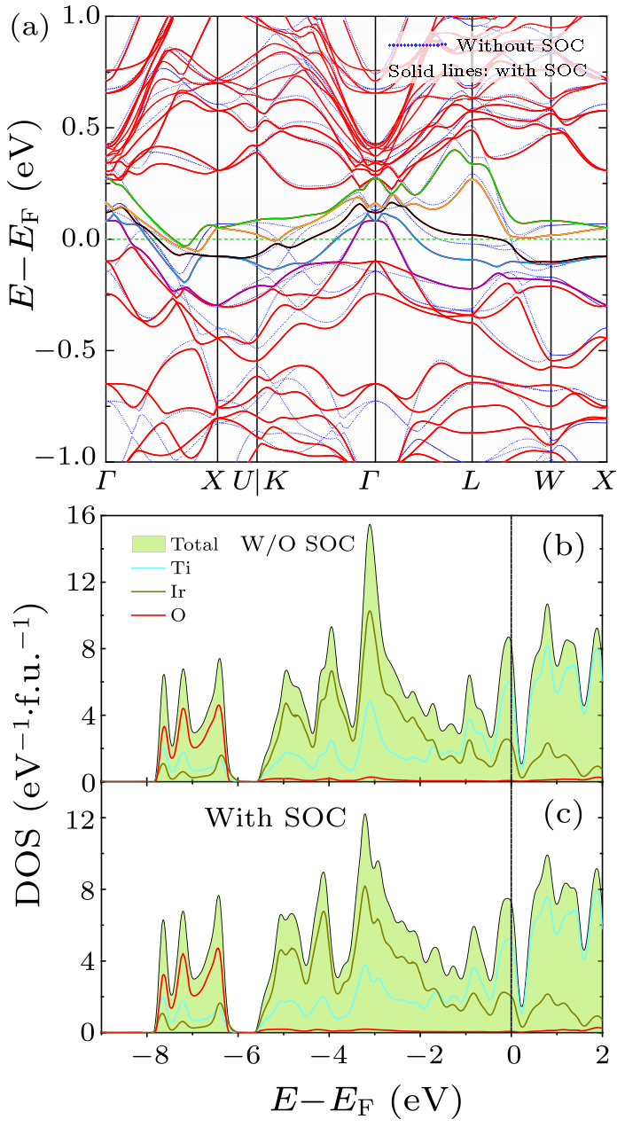
Fig. 4. (a) Electronic band structures of Ti$_4$Ir$_2$O from DFT calculation. Dotted lines show the results without SOC, while the SOC results are shown as solid lines. Solid lines in colors other than red indicate the bands crossing the Fermi level. (b) Projected DOS without SOC. (c) Projected DOS with SOC.
Results from the first principles calculation are shown in Fig. 4, with electronic band structures in Fig. 4(a) and DOS in Figs. 4(b) and 4(c). Both the scalar relativistic (w/o SOC) and the fully relativistic (with SOC) results are shown. In both cases, there are five bands crossing the Fermi level, consistent with the metallic nature of Ti$_4$Ir$_2$O. The existence of multiple bands crossing $E_{\rm F}$ also makes multigap superconductivity plausible. Notice that the energy dispersion near $E_{\rm F}$ is dramatically changed when SOC is turned on. For example, band splitting occurs along the $\varGamma$–$X$, $\varGamma$–$K$, and $L$–$W$ lines. This makes the Fermi surface topology very different when considering SOC (see Fig. S5). Most absorbingly, nesting between the electron-like and hole-like pockets becomes prominent when SOC is turned on. The Barder analysis was based on the converged charge densities, resulting in a valence configuration of Ti$^{1.32+}_4$Ir$^{1.94-}_2$O$^{1.40-}$. This means charge transferring from Ti to Ir and O. The charge density and electron localization function (ELF) maps are shown in Fig. S4, from which ionic Ti–O bonds and metallic Ti–Ir bonds can be identified. From the projected DOS, shown in Figs. 4(b) and 4(c), we note the states from O are absent near $E_{\rm F}$. While they hybridize with states from Ti at $\sim$$-5.6$ to $-2$ eV, indicating the formation of Ti–O bonds. DOS at $E_{\rm F}$ is slightly lowered with SOC, giving a theoretical $N'(E_{\rm F}) = 7.26$ eV$^{-1}$ per f.u. This value is comparable with the one calculated from $\gamma$. The slightly enhancement of experimental $N(E_{\rm F})$ is possibly due to the electron-electron correlations. Notice that $E_{\rm F}$ locates near a pronounced peak of DOS, which arises from the relatively flat energy dispersion of the bands near $E_{\rm F}$. After the projection to each atomic orbital, we find that DOS at $E_{\rm F}$ originates mainly from the Ti-3$d$ orbitals, with minor contributions from the Ir-5$d$ components. Discussion and Conclusion. First we would like to discuss the stoichiometry of Ti$_4$Ir$_2$O, because $\eta$-carbide type phases frequently host vacancies on the interstitial sites.[24,25] According to the preparation procedure and the XRD results, however, the oxygen vacancies should be very close to zero. On the other hand, there should be a tiny amount of oxygen vacancies, since samples prepared at 1250 K were found to host smaller lattices and an enhanced $T_{\rm c}$ of 5.7 K (see the Supplementary Material). In $\eta$-carbide type suboxides, the lattice shrinks when more oxygen is incorporated, as observed in Zr$_4$Rh$_2$O$_{0.6}$.[24] This means that the oxygen contents in the 5.7 K samples are larger. The change of $T_{\rm c}$ should be attributed to the slight non-stoichiometry of Ti$_4$Ir$_2$O, given that DOS has a steep slope at $E_{\rm F}$. In other words, a small amount of electron doping can dramatically change the value of $N(E_{\rm F})$. For example, $N(E_{\rm F})$ would be reduced to 6.80 eV$^{-1}$ per f.u. if 10% oxygen vacancies were introduced (assuming a rigid band model). The evolution of $T_{\rm c}$ upon vacancies requires detailed doping studies in the future. Next we focus on the origin of the large $H_{\rm c2}$. One possible cause of the enhancement of $H_{\rm c2}$ is the spin-triplet component in the order parameter, which can be induced by non-centrosymmetric crystal structures.[7,8] However, this should not be the case since Ti$_4$Ir$_2$O hosts a centrosymmetric crystal structure. Another possibility of enhancement due to anisotropy, as observed in many low-dimensional superconductors, such as Li$_{0.9}$Mo$_6$O$_{17}$,[52] LaO$_{0.5}$F$_{0.5}$BiS$_2$,[15] La$_2$IRu$_2$,[53] and K$_2$Mo$_3$As$_3$,[54] is also ruled out. Because both the crystal structure and the Fermi surfaces (see Fig. S5) are clearly three-dimensional. In heavy fermion superconductors, a reduction of $g$ factor can cause a violation of the Pauli limit.[55] To see whether there is a strong correlation, a fit to the normal state magnetization data is carried out based on $\chi(T)=\chi_0 + C/(T-\theta)$, giving a temperature-independent term of $\chi_0 = 1.73 \times 10^{-3}$ emu$\cdot$mol$^{-1}$. After subtracting the core diamagnetic contributions from Ti$^{4+}$, Ir$^{4+}$, and O$^{2-}$, we obtain an estimation of the Pauli paramagnetic susceptibility $\chi_{_{\scriptstyle \rm P}} \sim 1.84 \times 10^{-3}$ emu$\cdot$mol$^{-1}$. Therefore, the Wilson ratio $R_{\rm W} = \pi^2k_{\scriptscriptstyle{\rm B}}^2\chi_{_{\scriptstyle \rm P}}/(3\gamma\mu_{\scriptscriptstyle{\rm B}}^2) \sim 3.9$. Such a large $R_{\rm W}$ indicates the existence of strong electron correlation and/or an underlying magnetic order.[56,57] The strong electron correlation is further evidenced by the Kadowaki–Woods ratio $A/\gamma^2 = 9.0 \times 10^{-6}\,µ\Omega\cdot$cm/(mJ$\cdot$mol$^{-1}\cdot$K$^{-1}$)$^2$, which is comparable with those in heavy fermion systems (for instance, $1.0 \times 10^{-5}\,µ\Omega\cdot$cm/(mJ$\cdot$mol$^{-1}\cdot$K$^{-1}$)$^2$ for UPt$_3$[5] and CeCu$_2$Si$_2$[58]). It is also probably the cause for the enhancement of $\gamma$ compared with the theoretical value. The strong correlation might cause an enhancement of the electronic effective mass ($m^*$) and a reduction of $g$ factor, which would result in a large $H_{\rm c2}$. However, there is currently no clear experimental evidence for such an assumption. Further studies are needed to elucidate this issue. Finally, since the Pauli limit is based on the BCS weak coupling gap value of 1.76$k_{\scriptscriptstyle{\rm B}}T_{\rm c}$, a strong coupling can also enhance it. In our case, $\varDelta_1/k_{\scriptscriptstyle{\rm B}}T_{\rm c} = 3.10$ is indeed beyond the BCS weak coupling limit. However, superconductors with similar coupling strength, such as the A15 compounds[41,42] or SrPt$_3$P,[43] do not necessarily host a large $H_{\rm c2}$. The violation of Pauli limit in Ti$_4$Ir$_2$O is possibly due to a combination of the strong-coupled superconductivity and the spin-orbit scattering, while unconventional superconductivity cannot be excluded. To summarize, we have reported a detailed investigation of superconductivity in Ti$_4$Ir$_2$O. As a strong-coupled superconductor with $T_{\rm c} = 5.1 \sim 5.7$ K, Ti$_4$Ir$_2$O exhibits many intriguing properties. It has a large $\mu_0H_{\rm c2}(0)$ of 16.45 T, which is beyond the Pauli paramagnetic limit. A multigap superconductivity is suggested by the temperature dependence of $H_{\rm c2}$, the heat capacity measurements, and the DFT calculations. Moreover, a strong electron correlation in Ti$_4$Ir$_2$O, which is comparable with typical heavy fermion superconductors, is revealed by the large values of the Wilson ratio and the Kadowaki–Woods ratio, as well as the relatively large Sommerfeld coefficient ($\gamma$). These results make Ti$_4$Ir$_2$O a rare example to study the interplay between strong electron correlation and multigap superconductivity. We note that these results also strongly suggest unconventional superconductivity. Questions like whether there are spin fluctuations or a direct observation of the multigap feature through spectroscopy methods are still open, calling for further studies. Given the fact that there are numerous $\eta$-carbide type compounds, most of which are not systematically investigated for their transport properties, detailed studies in this structural family may flourish in the near future. Note. During the preparation of the manuscript, we note an independent report (published in November 2021) of superconductivity in Ti$_4$Ir$_2$O by Ma et al.[59] The superconducting parameters determined there are in agreement fairly well with ours. Acknowledgments. This work was supported by the National Natural Science Foundation of China (Grant Nos. 12074414 and 11774402), the National Key Research and Development of China (Grant No. 2018YFA0704200), and the Strategic Priority Research Program of Chinese Academy of Sciences (Grant No. XDB25000000).
References To use or not to use cool superconductors?45.5-tesla direct-current magnetic field generated with a high-temperature superconducting magnetSuperconductivity in the A15 structurePossibility of Coexistence of Bulk Superconductivity and Spin Fluctuations in U Pt 3 Upper Critical Fields and Anisotropy of BaFe1.9Ni0.1As2 Single CrystalsHeavy Fermion Superconductivity and Magnetic Order in Noncentrosymmetric C e P t 3 S i Gap symmetry of the noncentrosymmetric superconductor W 3 Al 2 C Superconductivity in Quasi-One-Dimensional K 2 Cr 3 As 3 with Significant Electron CorrelationsNMR Investigation of the Quasi-One-Dimensional Superconductor K 2 Cr 3 As 3 Unconventional superconductivity in quasi-one-dimensional Rb 2 Cr 3 As 3 Pauli-limit violation and re-entrant superconductivity in moiré grapheneSuperconductivity at 6 K and the Violation of Pauli Limit in Ta 2 Pd x S 5Upper Critical Field Measurements up to 600 kG in PbMo 6 S 8Anisotropic two-gap superconductivity and the absence of a Pauli paramagnetic limit in single-crystalline LaO 0.5 F 0.5 BiS 2 A New Complex Eta-CarbideThe formation of η carbidesThe structures of the η-carbides Ni6Mo6C, Co6Mo6C, and Co6Mo6C2Phasen mit aufgef�lltem Ti2Ni-TypThermal expansion and compressibility of Co6W6CSynthesis, Structure, and Hydrogen-Sorption Properties of (Ti,Zr)4Ni2N x SubnitridesNano-structured nickel–molybdenum carbide catalyst for low-temperature water-gas shift reactionSuperconductivity in the η-carbide-type oxides Zr 4 Rh 2 O x Superconductivity with High Upper Critical Field in the Cubic Centrosymmetric η-Carbide Nb 4 Rh 2 C 1−δSuperconductivitySuperconductivity in zirconium-rhodium alloysEXPGUI , a graphical user interface for GSASSuperconductivity in a new T2-phase Mo5GeB2Effective Demagnetizing Factors of Diamagnetic Samples of Various ShapesQUANTUM ESPRESSO: a modular and open-source software project for quantum simulations of materialsAdvanced capabilities for materials modelling with Quantum ESPRESSOQ uantum ESPRESSO toward the exascaleRestoring the Density-Gradient Expansion for Exchange in Solids and SurfacesPseudopotentials periodic table: From H to PuCritic2: A program for real-space analysis of quantum chemical interactions in solidsMaximally localized Wannier functions for describing a topological phase transition in staneneWannier90 as a community code: new features and applicationsSuperconductivity in an intermetallic oxide Hf 3 Pt 4 Ge 2 O*Properties of boson-exchange superconductorsSaturation of the High-Temperature Normal-State Electrical Resistivity of SuperconductorsStrong Coupling Superconductivity at 8.4 K in an Antiperovskite Phosphide Sr Pt 3 P Electrons in transition metalsTemperature and Purity Dependence of the Superconducting Critical Field, H c 2 . IIMagnetoresistivity and H c 2 ( T ) in MgB 2 Pressure Induced Effects on the Fermi Surface of Superconducting 2 H NbSe 2 Possible multiband superconductivity in the quaternary carbide YRe 2 SiCEnhancement of the upper critical field by nonmagnetic impurities in dirty two-gap superconductorsTransition Temperature of Strong-Coupled SuperconductorsUpper Critical Magnetic Field far above the Paramagnetic Pair-Breaking Limit of Superconducting One-Dimensional Li 0.9 Mo 6 O 17 Single CrystalsSuperconductivity at 4.8 K and Violation of Pauli Limit in La 2 IRu 2 Comprising Ru Honeycomb LayerSuperconductivity at 10.4 K in a novel quasi-one-dimensional ternary molybdenum pnictide K2Mo3As3Superconducting Pairs with Extreme Uniaxial Anisotropy in URu 2 Si 2 Ferromagnetic cluster spin-glass behavior in PrRhSn 3 Strong electron-electron correlation in the antiperovskite compound GaCNi 3 Superconductivity in the Presence of Strong Pauli Paramagnetism: Ce Cu 2 Si 2 Group-9 Transition-Metal Suboxides Adopting the Filled-Ti 2 Ni Structure: A Class of Superconductors Exhibiting Exceptionally High Upper Critical Fields
[1] Gurevich A 2011 Nat. Mater. 10 255
[2] Hahn S, Kim K, Kim K, Hu X, Painter T, Dixon I, Kim S, Bhattarai K R, Noguchi S, Jaroszynski J, and Larbalestier D C 2019 Nature 570 496
[3] Stewart G 2015 Physica C 514 28
[4]Poole C K, Farach H A, and Creswick R J 1999 Handbook of Superconductivity (Amsterdam: Elsevier)
[5] Stewart G, Fisk Z, Willis J, and Smith J 1984 Phys. Rev. Lett. 52 679
[6] Tao Q, shen J Q, Li L J et al 2009 Chin. Phys. Lett. 26 097401
[7] Bauer E, Hilscher G, Michor H, Paul C, Scheidt E, Gribanov A, Seropegin Y, Noel H, Sigrist M, and Rogl P 2004 Phys. Rev. Lett. 92 027003
[8] Gupta R, Ying T, Qi Y, Hosono H, and Khasanov R 2021 Phys. Rev. B 103 174511
[9] Bao J K, Liu J Y, Ma C W, Meng Z H, Tang Z T, Sun Y L, Zhai H F, Jiang H, Bai H, Feng C M et al. 2015 Phys. Rev. X 5 011013
[10] Zhi H, Imai T, Ning F, Bao J K, and Cao G H 2015 Phys. Rev. Lett. 114 147004
[11] Tang Z T, Bao J K, Liu Y, Sun Y L, Ablimit A, Zhai H F, Jiang H, Feng C M, Xu Z A, and Cao G H 2015 Phys. Rev. B 91 020506
[12] Cao Y, Park J M, Watanabe K, Taniguchi T, and Jarillo-Herrero P 2021 Nature 595 526
[13] Lu Y, Takayama T, Bangura A F, Katsura Y, Hashizume D, and Takagi H 2014 J. Phys. Soc. Jpn. 83 023702
[14] Okuda K, Kitagawa M, Sakakibara T, and Date M 1980 J. Phys. Soc. Jpn. 48 2157
[15] Chan Y C, Yip K Y, Cheung Y W, Chan Y T, Niu Q, Kajitani J, Higashinaka R, Matsuda T D, Yanase Y, Aoki Y, Lai K T, and Goh S K 2018 Phys. Rev. B 97 104509
[16] Taylor A and Sachs K 1952 Nature 169 411
[17] Kuo K 1953 Acta Metall. 1 301
[18] Newsam J, Jacobson A, McCandlish L, and Polizzotti R 1988 J. Solid State Chem. 75 296
[19] Jeitschko W, Holleck H, Nowotny H, and Benesovsky F 1964 Monatsh. Chem. - Chem. Mon. 95 1004
[20] Dubrovinskaia N, Dubrovinsky L, Saxena S, Selleby M, and Sundman B 1999 J. Alloys Compd. 285 242
[21] Zavalii I, Verbovytskyi Y, Berezovets V, Shtender V, Pecharsky V, and Lyutyi P 2017 Mater. Sci. 53 306
[22] Nagai M, Zahidul A M, and Matsuda K 2006 Appl. Catal. A 313 137
[23]Ku H and Johnston D 1984 Chin. J. Phys. 22 59
[24] Ma K, Lago J, and von Rohr F O 2019 J. Alloys Compd. 796 287
[25] Ma K, Gornicka K, Lefèvre R, Yang Y, Rønnow H M, Jeschke H O, Klimczuk T, and von Rohr F O 2021 ACS Mater. Au 1 55
[26] Matthias B, Geballe T, and Compton V 1963 Rev. Mod. Phys. 35 1
[27] Zegler S 1965 J. Phys. Chem. Solids 26 1347
[28] Toby B 2001 J. Appl. Crystallogr. 34 210
[29] Ruan B B, Yang Q S, Zhou M H, Chen G F, and Ren Z A 2021 J. Alloys Compd. 868 159230
[30] Prozorov R and Kogan V G 2018 Phys. Rev. Appl. 10 014030
[31] Giannozzi P, Baroni S, Bonini N, Calandra M, Car R, Cavazzoni C, Ceresoli D, Chiarotti G L, Cococcioni M, Dabo I, Dal C A, de Gironcoli S, Fabris S, Fratesi G, Gebauer R, Gerstmann U, Gougoussis C, Kokalj A, Lazzeri M, Martin-Samos L, Marzari N, Mauri F, Mazzarello R, Paolini S, Pasquarello A, Paulatto L, Sbraccia C, Scandolo S, Sclauzero G, Seitsonen A P, Smogunov A, Umari P, and Wentzcovitch R M 2009 J. Phys.: Condens. Matter 21 395502
[32] Giannozzi P, Andreussi O, Brumme T, Bunau O, Nardelli M B, Calandra M, Car R, Cavazzoni C, Ceresoli D, Cococcioni M, Colonna N, Carnimeo I, Corso A D, de Gironcoli S, Delugas P, DiStasio R A, Ferretti A, Floris A, Fratesi G, Fugallo G, Gebauer R, Gerstmann U, Giustino F, Gorni T, Jia J, Kawamura M, Ko H Y, Kokalj A, Küçükbenli E, Lazzeri M, Marsili M, Marzari N, Mauri F, Nguyen N L, Nguyen H V, Otero-de-la-Roza A, Paulatto L, Poncé S, Rocca D, Sabatini R, Santra B, Schlipf M, Seitsonen A P, Smogunov A, Timrov I, Thonhauser T, Umari P, Vast N, Wu X, and Baroni S 2017 J. Phys.: Condens. Matter 29 465901
[33] Giannozzi P, Baseggio O, Bonfa P, Brunato D, Car R, Carnimeo I, Cavazzoni C, de Gironcoli S, Delugas P, Ruffino F F, Ferretti A, Marzari N, Timrov I, Urru A, and Baroni S 2020 J. Chem. Phys. 152 154105
[34] Perdew J P, Ruzsinszky A, Csonka G I, Vydrov O A, Scuseria G E, Constantin L A, Zhou X, and Burke K 2008 Phys. Rev. Lett. 100 136406
[35] Dal C A 2014 Comput. Mater. Sci. 95 337
[36] Otero-de-la-Roza A, Johnson E R, and Luana V 2014 Comput. Phys. Commun. 185 1007
[37] Fuhr J D, Roura-Bas P, and Aligia A A 2021 Phys. Rev. B 103 035126
[38] Pizzi G, Vitale V, Arita R, Bluegel S, Freimuth F, Geranton G, Gibertini M, Gresch D, Johnson C, Koretsune T, Ibanez-Azpiroz J, Lee H, Lihm J M, Marchand D, Marrazzo A, Mokrousov Y, Mustafa I J, Nohara Y, Nomura Y, Paulatto L, Ponce S, Ponweiser T, Qiao J, Thoele F, Tsirkin S S, Wierzbowska M, Marzari N, Vanderbilt D, Souza I, Mostofi A A, and Yates J R 2020 J. Phys.: Condens. Matter 32 165902
[39]Okamoto H, Massalski T et al. 1990 Binary Alloy Phase Diagrams (Materials Park, OH: ASM International)
[40] Xu C, Wang H, Tian H, Shi Y, Li Z A, Xiao R, Shi H, Yang H, and Li J 2021 Chin. Phys. B 30 077403
[41] Carbotte J 1990 Rev. Mod. Phys. 62 1027
[42] Fisk Z and Webb G 1976 Phys. Rev. Lett. 36 1084
[43] Takayama T, Kuwano K, Hirai D, Katsura Y, Yamamoto A, and Takagi H 2012 Phys. Rev. Lett. 108 237001
[44]Mott N F, Jones H, Jones H, and Jones H 1958 The Theory of the Properties of Metals and Alloys (Courier Dover Publications)
[45] Mott N F 1964 Adv. Phys. 13 325
[46] Werthamer N, Helfand E, and PC H 1966 Phys. Rev. 147 288
[47] Bud'ko S, Petrovic C, Lapertot G, Cunningham C, Canfield P, Jung M, and Lacerda A 2001 Phys. Rev. B 63 220503
[48] Suderow H, Tissen V, Brison J, Martı́nez J, and Vieira S 2005 Phys. Rev. Lett. 95 117006
[49] De Faria L R, Ferreira P P, Correa L E, Eleno L T, Torikachvili M S, and Machado A J 2021 Supercond. Sci. Technol. 34 065010
[50] Gurevich A 2003 Phys. Rev. B 67 184515
[51] McMillan W L 1968 Phys. Rev. 167 331
[52] Mercure J F, Bangura A F, Xu X, Wakeham N, Carrington A, Walmsley P, Greenblatt M, and Hussey N E 2012 Phys. Rev. Lett. 108 187003
[53] Ishikawa H, Wedig U, Nuss J, Kremer R K, Dinnebier R, Blankenhorn M, Pakdaman M, Matsumoto Y, Takayama T, Kitagawa K, and Takagi H 2019 Inorg. Chem. 58 12888
[54] Mu Q G, Ruan B B, Zhao K, Pan B J, Liu T, Shan L, Chen G F, and Ren Z A 2018 Sci. Bull. 63 952
[55] Altarawneh M, Harrison N, Li G, Balicas L, Tobash P, Ronning F, and Bauer E 2012 Phys. Rev. Lett. 108 066407
[56] Anand V K, Adroja D T, and Hillier A D 2012 Phys. Rev. B 85 014418
[57] Tong P, Sun Y P, Zhu X B, and Song W H 2006 Phys. Rev. B 73 245106
[58] Steglich F, Aarts J, Bredl C, Lieke W, Meschede D, Franz W, and Schafer H 1979 Phys. Rev. Lett. 43 1892
[59] Ma K, Lefèvre R, Gornicka K, Jeschke H O, Zhang X, Guguchia Z, Klimczuk T, and von Rohr F O 2021 Chem. Mater. 33 8722