Chinese Physics Letters, 2020, Vol. 37, No. 8, Article code 080502Express Letter Negative Thermal Transport in Conduction and Advection Liujun Xu (须留钧)* and Jiping Huang(黄吉平)* Affiliations Department of Physics, State Key Laboratory of Surface Physics, and Key Laboratory of Micro and Nano Photonic Structures (MOE), Fudan University, Shanghai 200438, China Received 2 July 2020; accepted 15 July 2020; published online 18 July 2020 Supported by the National Natural Science Foundation of China (Grant No. 11725521).
*Corresponding authors. Email: 13307110076@fudan.edu.cn; jphuang@fudan.edu.cn
Citation Text: Xu L J and Huang J P 2020 Chin. Phys. Lett. 37 080502    Abstract Negative refractive index has drawn a great deal of attention due to its unique properties and practical applications in wave systems. To promote the related physics in thermotics, here we manage to coin a complex thermal conductivity whose imaginary part corresponds to the real part of complex refractive index. Therefore, the thermal counterpart of negative refractive index is just negative imaginary thermal conductivity, which is featured by the opposite directions of energy flow and wave vector in thermal conduction and advection, thus called negative thermal transport herein. To avoid violating causality, we design an open system with energy exchange and explore three different cases to reveal negative thermal transport. We further provide experimental suggestions with a solid ring structure. All finite-element simulations agree with theoretical analyses, indicating that negative thermal transport is physically feasible. These results have potential applications such as designing the inverse Doppler effect in thermal conduction and advection. DOI:10.1088/0256-307X/37/8/080502 PACS:05.70.-a, 44.10.+i, 47.55.pb © 2020 Chinese Physics Society Article Text Negative refraction is one of the most attracting phenomena in wave systems, which was first revealed with simultaneously negative permeability and permittivity.[1] With the proposal of metal wire arrays[2] and split rings,[3] negative refractive index was soon designed and fabricated,[4–6] which gave birth to wide applications such as breaking diffraction limit.[7–9] One representative property of negative refractive index is the opposite directions of energy flow (or Poynting vector) and wave vector [see Fig. 1(a)]. Based on this property, related phenomena were revealed intensively, such as the inverse Doppler effect,[10] the inverse Cerenkov radiation,[11] and the abnormal Goos–Hanschen shift.[12]
cpl-37-8-080502-fig1.png
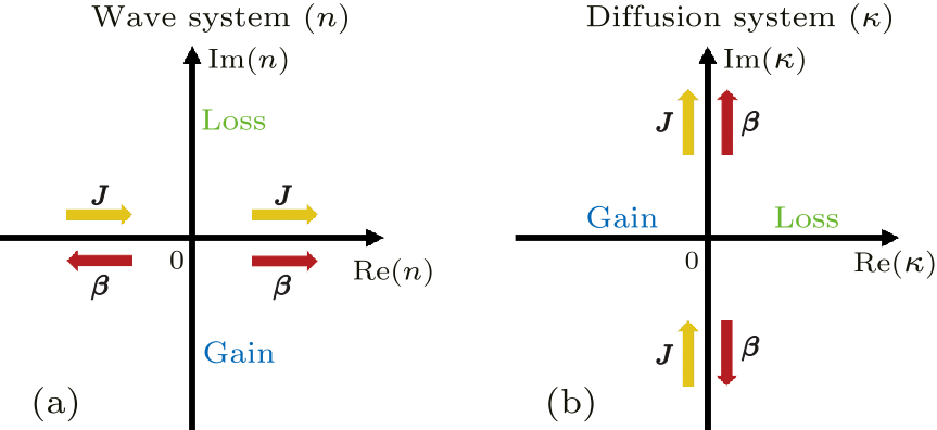
Fig. 1. Comparison between (a) wave system and (b) diffusion system. Here $n$ and $\kappa$ denote the complex refractive index and the complex thermal conductivity, respectively. ${\boldsymbol J}$ and ${\boldsymbol \beta}$ denote the energy flow and the wave vector, respectively.
Similar refractive phenomena were also studied with thermal wave generated by a time-periodic heat source.[13] Moreover, multilayered structures were also proposed to guide heat flow,[14–17] yielding practical applications such as thermal lens[18] and thermal cloaks.[19] These studies made an attempt to connect thermal phenomena and electromagnetic phenomena. However, some basic concepts are still ambiguous, especially the correspondence between thermal conductivity and refractive index. To promote the related physics in thermotics with a clear physical picture, here we manage to coin a complex thermal conductivity $\kappa$ as the thermal counterpart of complex refractive index $n$ (see Fig. 1). The imaginary part of complex thermal conductivity has an analogy of the real part of complex refractive index. Therefore, the thermal counterpart of negative refractive index is just negative imaginary thermal conductivity, which is characterized by the opposite directions of energy flux ${\boldsymbol J}$ and wave vector ${\boldsymbol \beta}$, thus called negative thermal transport. We design an open system with energy exchange to observe negative thermal transport, and further provide experimental suggestions with a three-dimensional solid ring structure. All theoretical analyses and finite-element simulations indicate that negative thermal transport is physical. Let us start from coining complex thermal conductivity. Thermal conduction-advection process is dominated by the famous equation $$ \rho C\frac{\partial T}{\partial t}+{\nabla}\cdot \left({-\sigma {\nabla}T+\rho C{\boldsymbol v}T} \right)=0,~~ \tag {1} $$ where $\rho$, $C$, $\sigma$, ${\boldsymbol v}$, $T$, and $t$ are the density, heat capacity, thermal conductivity, convective velocity, temperature, and time, respectively. Equation (1) indicates the energy conservation of thermal conduction and advection. We assume that the convective term $({\rho C{\boldsymbol v}T})$ results from the motion of solid, so density and heat capacity can be seen as two constants which do not depend on time or temperature.[20,21] Therefore, the mass and momentum conservations of thermal advection are naturally satisfied. To proceed, we apply a plane-wave solution for temperature,[20–22] $$ T=A_{0} {e}^{{i}\left({{\boldsymbol \beta }\cdot {\boldsymbol r}-\omega t} \right)}+T_{0},~~ \tag {2} $$ where $A_{0}$, ${\boldsymbol \beta}$, ${\boldsymbol r}$, $\omega$, and $T_{0}$ are the amplitude, wave vector, position vector, frequency, and reference temperature of wave-like temperature profile, respectively; ${i}=\sqrt {-1}$ is imaginary unit. Only the real part of Eq. (2) makes sense. We substitute Eq. (2) into Eq. (1), and derive a dispersion relation as follows: $$ \omega ={\boldsymbol v}\cdot {\boldsymbol \beta }-{i}\frac{\sigma \beta^{2}}{\rho C}.~~ \tag {3} $$ With the wave-like temperature profile described by Eq. (2), we can derive ${\nabla}T={i}{\boldsymbol \beta }T$ ($T_{0}$ is neglected for brevity). Then, Eq. (1) can be rewritten as $$ \rho C\frac{\partial T}{\partial t}+{\nabla}\cdot \left({-{i}\sigma {\boldsymbol \beta }T+\rho C{\boldsymbol v}T} \right)=0.~~ \tag {4} $$ With the mass conservation of thermal advection, we can obtain ${\nabla}\cdot ({\rho {\boldsymbol v}})=0$ or ${\nabla}\cdot {\boldsymbol v}=0$ (with $\rho$ being a constant). Meanwhile, ${\boldsymbol \beta}$ is a constant vector, so Eq. (4) can be reduced to $$ \rho C\frac{\partial T}{\partial t}-{i}\sigma {\boldsymbol \beta }\cdot {\nabla}T+\rho C{\boldsymbol v}\cdot {\nabla}T=0,~~ \tag {5} $$ which can be further reduced with ${\nabla}T={i}{\boldsymbol \beta }T$ to $$ \rho C\frac{\partial T}{\partial t}+\sigma \beta^{2}T+{i}\rho C{\boldsymbol v}\cdot {\boldsymbol \beta }T=0.~~ \tag {6} $$ Now, it is natural to coin a complex thermal conductivity $\kappa$ as $$ \kappa =\sigma +{i}\frac{\rho C{\boldsymbol v}\cdot {\boldsymbol \beta }}{{\beta }^{2}},~~ \tag {7} $$ with which Eq. (6) can be simplified to $$ \rho C\frac{\partial T}{\partial t}+\kappa \beta^{2}T=0.~~ \tag {8} $$ With ${\nabla}T={i}{\boldsymbol \beta }T$, Eq. (8) is equivalent to the familiar equation of thermal conduction, $$ \rho C\frac{\partial T}{\partial t}+{\nabla}\cdot \left({-\kappa {\nabla}T} \right)=0.~~ \tag {9} $$ Clearly, the thermal conduction-advection equation (1) is converted to the complex thermal conduction equation (9) with a complex thermal conductivity (7). Although thermal conductivity is generally defined by fixing moving parts (advection) as zero, here advection can be mathematically regarded as a complex form of conduction. That is, conduction and advection are mathematically unified within a conductive framework (despite different physical mechanisms). Therefore, coining complex thermal conductivity makes sense as long as treating advection as a complex form of conduction. Substituting Eq. (2) into Eq. (9), we can derive the dispersion relation $$ \omega =-{i}\frac{\kappa \beta^{2}}{\rho C}={\boldsymbol v}\cdot {\boldsymbol \beta }-{i}\frac{\sigma \beta^{2}}{\rho C},~~ \tag {10} $$ which is in accordance with the result of Eq. (3), indicating that complex thermal conductivity is physical. To understand the complex frequency $\omega$, we substitute Eq. (10) into Eq. (2), and the wave-like temperature profile becomes $$ T=A_{0} {e}^{{\rm Im}(\omega)t}{e}^{{i}\left[ {{\boldsymbol \beta }\cdot {\boldsymbol r}-{\rm Re}(\omega)t} \right]}+T_{0}.~~ \tag {11} $$ Obviously, ${\rm Re}(\omega)$ and ${\rm Im}(\omega)$ determine propagation and dissipation, respectively. Meanwhile, ${\rm Re}(\omega)$ and ${\rm Im}(\omega)$ are related to ${\rm Im}(\kappa)$ and ${\rm Re}(\kappa)$, respectively. In other words, ${\rm Re}(\kappa)$ and ${\rm Im}(\kappa)$ are related to dissipation and propagation, respectively. The physical connotation can be clearly understood with Fig. 1(b). Positive (or negative) ${\rm Re}(\kappa)$ means loss (or gain), indicating the amplitude decrement (or increment) of wave-like temperature profile. ${\rm Im}(\kappa)$ is of our interest, which is discussed later. We further confirm complex thermal conductivity in a thermal conduction-advection system with COMSOL MULTIPHYSICS (http://www.comsol.com/). The system is shown in Fig. 2(a), which has width $L$ and height $H$. Left and right ends are set under a periodic boundary condition. Then, the wave vector can only take on discrete values, say, $\beta =2\pi m/L$ with $m$ being any positive integers. We take on $m=5$, and initial temperature is set at $T=40\cos (\beta x)+323$ K [see Figs. 2(b) and 2(f)]. We discuss two cases with ${\boldsymbol v}|| {\boldsymbol \beta}$ [see Figs. 2(b)–2(e)] and ${\boldsymbol v}\bot {\boldsymbol \beta}$ [see Figs. 2(f)–2(i)]. When ${\boldsymbol v}|| {\boldsymbol \beta}$, ${\rm Im}(\kappa)$ appears due to ${\boldsymbol v}\cdot {\boldsymbol \beta }\ne 0$, as predicted by Eq. (7). Therefore, propagation occurs and the period of wave-like temperature profile is $t_{0} =2\pi /{\rm Re}(\omega)=2\pi /({\boldsymbol v}\cdot {\boldsymbol \beta })=100$ s, as predicted by Eq. (10). The wave-like temperature profiles at $t=0.5t_{0} =50$ s and $t=t_{0} =100$ s are shown in Figs. 2(c) and 2(d), respectively. The temperature distributions along the $x$ axis in Figs. 2(b)–2(d) are plotted in Fig. 2(e). Clearly, the wave-like temperature profile has amplitude decrement because of the positive ${\rm Re}(\kappa)$. Meanwhile, the wave-like temperature profile propagates along the $x$ axis due to the positive ${\rm Im}(\kappa)$. After propagating for a period (100 s), the wave-like temperature profile approximately gains a phase difference of $2\pi$, thus going back to the initial position [see Figs. 2(b) and 2(d)]. When ${\boldsymbol v}\bot {\boldsymbol \beta}$, ${\rm Im}(\kappa)$ vanishes due to ${\boldsymbol v}\cdot {\boldsymbol \beta }=0$. Therefore, propagation does not occur, and the period is $t_{0} =2\pi /{\rm Re}(\omega)=2\pi /({\boldsymbol v}\cdot {\boldsymbol \beta })=\infty$ s, as predicted by Eq. (10). The wave-like temperature profiles at $t=50$ s and $t=100$ s are presented in Figs. 2(g) and 2(h), respectively. The temperature distributions along the $x$ axis in Figs. 2(f)–2(h) are plotted in Fig. 2(i). The wave-like temperature profile has also amplitude decrement due to the positive ${\rm Re}(\kappa)$. However, the wave-like temperature profile does not propagate because of the zero ${\rm Im}(\kappa)$. Therefore, the behaviors of thermal conduction and advection can be well described by using complex thermal conductivity. When wave vector and convective velocity are with an arbitrary angle $\theta$, the velocity component $v\cos \theta$ contributes to propagation.
cpl-37-8-080502-fig2.png
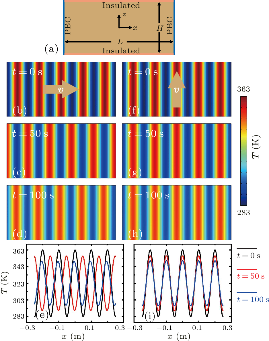
Fig. 2. (a) Schematic diagram. Temperature evolutions with (b)–(e) ${\boldsymbol v}|| {\boldsymbol \beta}$ and (f)–(i) ${\boldsymbol v}\bot {\boldsymbol \beta}$. Parameters: $L=0.5$ m, $H=0.25$ m, $\rho C=10^{6}$ J$\cdot$m$^{-3}$K$^{-1}$, $\sigma =1$ W$\cdot$m$^{-1}$K$^{-1}$, and $v=1$ mm/s. PBC: periodic boundary condition.
We further discuss the energy flow in Figs. 2(b)–2(d). Relative energy flow ${\boldsymbol J}'$ can be calculated with periodicity average, $$ {\boldsymbol J}'=\frac{1}{\lambda }\int_0^\lambda {\left({-\kappa {\nabla}T} \right)} dx=0,~~ \tag {12} $$ where $\lambda =2\pi /\beta$ is wavelength. Here we only take on the real part of ${\boldsymbol J}'$ because the imaginary part does not make sense. Although conductive flow is irrelevant to reference temperature, convective flow $({\rho C{\boldsymbol v}T})$ is closely associated with reference temperature.[23–27] Therefore, absolute energy flow ${\boldsymbol J}$ is $$ {\boldsymbol J}=\rho C{\boldsymbol v}T_{0}.~~ \tag {13} $$ In what follows, we discuss absolute energy flow and neglect the expression of absolute for brevity. Clearly, ${\boldsymbol J}$ and ${\boldsymbol v}$ have the same direction. In other words, only thermal advection contributes to energy flow. As we can imagine from Figs. 2(b)–2(d), thermal advection results in the motion of wave-like temperature profile, so the direction of wave vector ${\boldsymbol \beta}$ follows that of convective velocity ${\boldsymbol v}$, yielding positive thermal transport [${\rm Im}(\kappa)>0$; see Fig. 1(b)]. To some extent, positive thermal transport is the result of causality, so negative thermal transport [${\rm Im}(\kappa) < 0$; see Fig. 1(b)] is unique.
cpl-37-8-080502-fig3.png
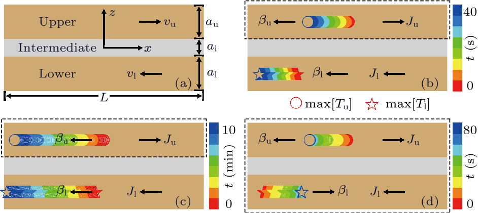
Fig. 3. Two-dimensional negative thermal transport. (a) Schematic diagram with $a_{\rm u} =a_{\rm l} =2$ mm, $a_{\rm i} =1$ mm, $L=0.5$ m, $\sigma_{\rm u} =\sigma_{\rm l} =10$ W$\cdot$m$^{-1}$K$^{-1}$, $\sigma_{\rm i} =0.1$ W$\cdot$m$^{-1}$K$^{-1}$, and $\rho_{\rm u} C_{\rm u} =\rho_{\rm l} C_{\rm l} =\rho_{\rm i} C_{\rm i} =10^{6}$ J$\cdot$m$^{-3}$K$^{-1}$. These parameters lead to $g/\beta =4$ mm/s. (b) $v_{\rm u} =-v_{\rm l} =5$ mm/s. (c) $v_{\rm u} =0.5$ mm/s and $v_{\rm l} =-1.5$ mm/s. (d) $v_{\rm u} =-v_{\rm l} =1$ mm/s. Circles and stars denote the trajectories of max[$T_{\rm u}$] and max[$T_{\rm l}$], respectively.
It may be difficult to reveal negative thermal transport in an isolated system like Fig. 2(a), so we consider an open system [see Fig. 3(a)], where an intermediate layer allows heat exchange between upper and lower layers. The complex thermal conductivities of the upper layer ($\kappa_{\rm u}$) and the lower layer ($\kappa_{\rm l}$) are expressed as $$ \kappa_{\rm u} =\sigma_{\rm u} +{i}\frac{\rho_{\rm u} C_{\rm u} {\boldsymbol v}_{\rm u} \cdot {\boldsymbol \beta }_{\rm u} }{{\beta }_{\rm u}^{2}},~~ \tag {14a} $$ $$ \kappa_{\rm l} =\sigma_{\rm l} +{i}\frac{\rho_{\rm l} C_{\rm l} {\boldsymbol v}_{\rm l} \cdot {\boldsymbol \beta }_{\rm l} }{{\beta }_{\rm l}^{2}},~~ \tag {14b} $$ where the subscripts u and l denote the parameters in the upper and lower layers, respectively. We set the wave-like temperature profiles in the upper layer $T_{\rm u}$ and in the lower layer $T_{\rm l}$ as $$ T_{\rm u} =A_{\rm u} {e}^{{i}\left({{\boldsymbol \beta }_{\rm u} \cdot {\boldsymbol x}-\omega t} \right)}+T_{0},~~ \tag {15a} $$ $$ T_{\rm l} =A_{\rm l} {e}^{{i}\left({{\boldsymbol \beta }_{\rm l} \cdot {\boldsymbol x}-\omega t} \right)}+T_{0}.~~ \tag {15b} $$ The heat exchange between the upper and lower layers is along the $z$ axis, which is not of our concern. Therefore, the energy flows along the $x$ axis in the upper layer ${\boldsymbol J}_{\rm u}$ and in the lower layer ${\boldsymbol J}_{\rm l}$ can be calculated by $$ {\boldsymbol J}_{\rm u} =\rho_{\rm u} C_{\rm u} {\boldsymbol v}_{\rm u} T_{0},~~ \tag {16a} $$ $$ {\boldsymbol J}_{\rm l} =\rho_{\rm l} C_{\rm l} {\boldsymbol v}_{\rm l} T_{0}.~~ \tag {16b} $$ Clearly, the directions of energy flow in the upper and lower layers are opposite due to ${\boldsymbol v}_{\rm u} =-{\boldsymbol v}_{\rm l}$. The thermal conduction-advection processes in the upper and lower layers can be described by the complex thermal conduction equations $$ \rho_{\rm u} C_{\rm u} \frac{\partial T_{\rm u}}{\partial t}+{\nabla}\cdot \left({-\kappa_{\rm u} {\nabla}T_{\rm u} } \right)=s_{\rm u},~~ \tag {17a} $$ $$ \rho_{\rm l} C_{\rm l} \frac{\partial T_{\rm l}}{\partial t}+{\nabla}\cdot \left({-\kappa_{\rm l} {\nabla}T_{\rm l} } \right)=s_{\rm l},~~ \tag {17b} $$ where $s_{\rm u}$ and $s_{\rm l}$ are the two heat sources, reflecting the heat exchange between the upper and lower layers.[20,21] Since the three layers in Fig. 3(a) are thin enough, i.e., $\left({L\gg a_{\rm u,i,l} } \right)$, the temperature variance along the $z$ axis can be neglected, yielding $\partial^{2}T/\partial z^{2}=0$. The energy flow from the lower layer to the upper layer $j_{\rm u}$ can be calculated by $j_{\rm u} =-\sigma_{\rm i} (T_{\rm u} -T_{\rm l})/a_{\rm i}$, where $\sigma_{\rm i}$ and $a_{\rm i}$ are the thermal conductivity and width of stationary intermediate layer, respectively. It is also reasonable to suppose that energy flow is uniformly distributed in the upper layer due to thin thickness, so the heat source in the upper layer $s_{\rm u}$ can be expressed as $s_{\rm u} =j_{\rm u} /a_{\rm u} =-\sigma_{\rm i} ({T_{\rm u} -T_{\rm l} })/ ({a_{\rm i} a_{\rm u} })$, where $a_{\rm u}$ is the width of upper layer. Similarly, the heat source in lower layer $s_{\rm l}$ can be derived as $s_{\rm l} =j_{\rm l} /a_{\rm l} =-\sigma_{\rm i} ({T_{\rm l} -T_{\rm u} })/({a_{\rm i} a_{\rm l} })$, where $a_{\rm l}$ is the width of lower layer. With these analyses, Eqs. (17a) and (17b) can be reduced to $$ \rho_{\rm u} C_{\rm u} \frac{\partial T_{\rm u}}{\partial t}-\kappa_{\rm u} \frac{\partial^{2}T_{\rm u}}{\partial x^{2}}=h_{\rm u} \left({T_{\rm l} -T_{\rm u} } \right),~~ \tag {18a} $$ $$ \rho_{\rm l} C_{\rm l} \frac{\partial T_{\rm l}}{\partial t}-\kappa_{\rm l} \frac{\partial^{2}T_{\rm l}}{\partial x^{2}}=h_{\rm l} \left({T_{\rm u} -T_{\rm l} } \right),~~ \tag {18b} $$ where $h_{\rm u} =\sigma_{\rm i} /({a_{\rm i} a_{\rm u} })$ and $h_{\rm l} =\sigma_{\rm i} /({a_{\rm i} a_{\rm l} })$, reflecting the exchange rate of heat energy. We take on the same material parameters of the upper and lower layers, say, $\sigma_{\rm u} =\sigma_{\rm l} ({=\sigma })$, $\rho_{\rm u} C_{\rm u} =\rho_{\rm l} C_{\rm l} ({=\rho C})$, $a_{\rm u} =a_{\rm l} ({=a})$, and $h_{\rm u} =h_{\rm l} ({=h})$. We also suppose ${\boldsymbol v}_{\rm u} =-{\boldsymbol v}_{\rm l} ({={\boldsymbol v}})$ and ${\boldsymbol \beta }_{\rm u} ={\boldsymbol \beta }_{\rm l} ({={\boldsymbol \beta }})$, thus yielding $\kappa_{\rm u} =\bar{{\kappa }}_{\rm l} ({=\kappa })$, where $\bar{{\kappa }}_{\rm l}$ is the conjugate of $\kappa_{\rm l}$. Substituting Eq. (15) into Eq. (18) yields an eigenequation ${\hat{{H}}}{\boldsymbol \psi =}\omega {\boldsymbol \psi}$, where the Hamiltonian ${\hat{{H}}}$ reads $$ {\hat{{H}}}=\left[ {{ \begin{array}{*{20}c} {-{i}\left({g+\eta \beta^{2}} \right)} \hfill & {{i}g} \hfill \\ {{i}g} \hfill & {-{i}\left({g+\bar{{\eta }}\beta^{2}} \right)} \hfill \\ \end{array} }} \right],~~ \tag {19} $$ where $\eta =\kappa /\left({\rho C} \right)$ and $g=h/\left({\rho C} \right)$. The eigenvalue of Eq. (19) is $$ \omega_{\pm } =-{i}\Big[ {g+{\rm Re}(\eta)\beta^{2}\pm \sqrt {g^{2}-{\rm Im}^{2}(\eta)\beta^{4}} }\,\Big],~~ \tag {20} $$ where ${\rm Re}(\eta)=\sigma /({\rho C})$ and ${\rm Im}(\eta)\beta^{2}=v\beta$. With Eq. (20), we can obtain three different cases of negative thermal transport. We discuss the first case with $g^{2}-{\rm Im}^{2}(\eta)\beta^{4} < 0$, say, $v>g/\beta$. The corresponding eigenvector is $$ {\boldsymbol \psi }_{+} =\big[ {1,{e}^{{i}\pi /2-\delta }} \big]^{\varsigma },~~ \tag {21a} $$ $$ {\boldsymbol \psi }_{-} =\big[ {1,{e}^{{i}\pi /2+\delta }} \big]^{\varsigma },~~ \tag {21b} $$ where $\delta =\cosh^{-1}[ {{\rm Im}(\eta)\beta^{2}/g}]$, and $\varsigma$ denotes transpose. The eigenvectors in Eqs. (21a) and (21b) indicate that the wave-like temperature profiles in the upper and lower layers move with a constant phase difference of $\pi /2$ but with different amplitudes. We take on $\beta =2\pi m/L$ with $m=1$ in the following. The initial wave-like temperature profiles in the upper and lower layers are set as the eigenvector described by Eq. (21b), say, $T_{\rm u} =40\cos (\beta x)+323$ K and $T_{\rm l} ={e}^{\delta }40\cos (\beta x+\pi /2)+323$ K. We track the motion of maximum temperature in the upper and lower layers, max[$T_{\rm u}$] and max[$T_{\rm l}$], to observe the directions of wave vector. Since the amplitude of the wave-like temperature profile in the lower layer (with ${e}^{\delta }>1$) is larger than that in the upper layer, the directions of wave vector in the upper and lower layers are both leftward. Therefore, negative thermal transport occurs in the upper layer, and the transport in the lower layer is still positive [see Fig. 3(b)]. We discuss the second case with $g^{2}-{\rm Im}^{2}(\eta)\beta^{4}>0$, say, $0 < v < g/\beta$. The corresponding eigenvector is $$ {\boldsymbol \psi }_{+} =\big[ {1,{e}^{{i}({\pi -\alpha })}} \big]^{\varsigma },~~ \tag {22a} $$ $$ {\boldsymbol \psi }_{-} =\big[ {1,{e}^{{i}\alpha }} \big]^{\varsigma },~~ \tag {22b} $$ where $\alpha {\rm ={\sin}}^{-1} [ {{\rm Im} (\eta)\beta^{2}/g}]$. The eigenvectors in Eq. (22) indicate that the wave-like temperature profiles in the upper and lower layers are motionless with a constant phase difference of $\pi -\alpha$ or $\alpha$. To make the wave-like temperature profiles move, we give the system a reference velocity ${\boldsymbol v}_{0}$, resulting in ${\boldsymbol v}_{\rm u} ={\boldsymbol v}_{\rm u} '+{\boldsymbol v}_{0}$ and ${\boldsymbol v}_{\rm l} ={\boldsymbol v}_{\rm l} '+{\boldsymbol v}_{0}$, where ${\boldsymbol v}_{\rm u} '$ and ${\boldsymbol v}_{\rm l} '$ are original convective velocities. This operation does not affect the essence of eigenvectors in Eqs. (22a) and (22b), and only gives a reference velocity ${\boldsymbol v}_{0}$ to wave-like temperature profiles. We set the initial wave-like temperature profiles in the upper and lower layers to be the eigenvector described by Eq. (22b), say, $T_{\rm u} =40\cos (\beta x)+323$ K and $T_{\rm l} =40\cos (\beta x+\alpha)+323$ K. We also take on ${\boldsymbol v}_{0} =-0.5{\boldsymbol v}_{\rm u} '$, so the wave-like temperature profiles in upper and lower layers still maintain a constant phase difference of $\alpha$ but with leftward motion. The trajectories of max[$T_{\rm u}$] and max[$T_{\rm l}$] are presented in Fig. 3(c). Clearly, negative thermal transport occurs in upper layer. These two cases are both related to eigenvectors, indicating that negative thermal transport does occur in one layer (say, upper layer). However, if we regard the upper and lower layers as a whole, thermal transport will be still positive. To go further, we explore the third case which is related to non-eigenvectors and their dynamics, to reveal negative thermal transport in both the upper and lower layers. For this purpose, we set the initial wave-like temperature profiles by adding the eigenvector described by Eq. (22b) with an extra phase $\gamma$, say, ${\boldsymbol \psi }_{-} '=\left[ {1,{e}^{{i}\left({\alpha +\gamma } \right)}} \right]^{\varsigma}$, yielding $T_{\rm u} =40\cos (\beta x)+323$ K and $T_{\rm l} =40\cos (\beta x+\alpha +\gamma)+323$ K. In this way, even if we do not give a reference velocity to the system, the wave-like temperature profile still moves for reaching eigenvector. One principle of evolution route is to make temperature profile decay as slowly as possible. Therefore, the eigenvector ${\boldsymbol \psi }_{+}$ with a phase difference of $\pi -\alpha$ described by Eq. (22a) becomes a key due to its large decay rate [say, the $\omega_{+}$ of Eq. (20)]. The evolution route should try to avoid ${\boldsymbol \psi }_{+}$ to survive longer. When $\gamma \in \left({0,\pi -2\alpha } \right)$, negative thermal transport will not make the temperature profile go through ${\boldsymbol \psi }_{+}$, but positive thermal transport will make the temperature profile go through ${\boldsymbol \psi }_{+}$ twice. Therefore, evolution route naturally chooses negative thermal transport in both the upper and lower layers to decay more slowly [see Fig. 3(d)]. Nevertheless, after reaching eigenvector, the wave-like temperature profile keeps motionless, so negative thermal transport is no longer in existence. In other words, negative thermal transport is transient in both the upper and lower layers.
cpl-37-8-080502-fig4.png
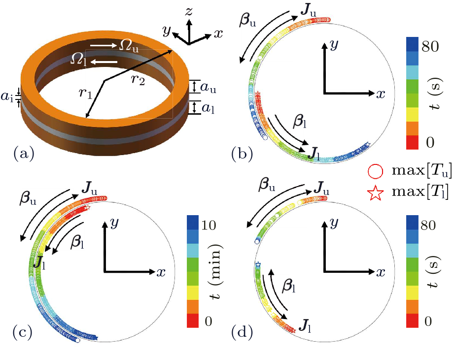
Fig. 4. Experimental suggestions with a three-dimensional solid ring structure. (a) Schematic diagram with $r_{1} =80$ mm and $r_{2} =82$ mm. Other parameters are kept the same as those for Fig. 3(a). (b) $\varOmega_{\rm u} =-\varOmega_{\rm l} =0.063$ rad/s. (c) $\varOmega_{\rm u} =0.006$ rad/s and $\varOmega_{\rm l} =-0.019$ rad/s. (d) $\varOmega_{\rm u} =-\varOmega_{\rm l} =0.013$ rad/s.
We also suggest experimental demonstration with a three-dimensional solid ring structure [see Fig. 4(a)], which can naturally meet the requirement of periodic boundary condition. The upper ring (with width $a_{\rm u}$) and the lower ring (with width $a_{\rm l}$) rotate with opposite angular velocities ($\varOmega_{\rm u}$ and $\varOmega_{\rm l}$), which are connected by a stationary intermediate layer (with width $a_{\rm i}$). The inner and outer radii of the ring structure are $r_{1}$ and $r_{2}$, respectively. Similar to two dimensions, we track max[$T_{\rm u}$] and max[$T_{\rm l}$] on the interior edge of the solid ring structure. The parametric settings for Figs. 4(b)–4(d) are basically the same as those for Figs. 3(b)–3(d), respectively. Therefore, the results are also similar. Negative thermal transport occurs in the upper ring of Figs. 4(b) and 4(c), and occurs in both the upper and lower rings of Fig. 4(d). The three-dimensional and two-dimensional results both agree well with the theoretical analyses, confirming the feasibility of negative thermal transport in thermal conduction and advection. Negative thermal transport may enlighten the inverse Doppler effect in thermal conduction and advection. Since energy flow is generated from energy source, a detector with opposite direction of energy flow is getting close to energy source. Positive thermal transport makes wave vector (which can be regarded as a thermal signal) follow the direction of energy flow. Therefore, the directions of detector and wave vector are also opposite, yielding frequency increment (the Doppler effect). However, negative thermal transport leads to the same directions of detector and wave vector. As a result, frequency decreases even though the detector is getting close to energy source (the inverse Doppler effect). These results may also provide guidance to extend transformation thermotics[28–30] to complex regime[31] and regulate thermal imaging.[32–37] Other thermal systems such as those with periodic structures[38–41] are also good candidates to explore negative thermal transport. Nevertheless, here we reveal negative thermal transport in an open system with energy exchange, so there is still a difference from wave systems where no energy exchange is required to realize negative refraction. Whether negative thermal transport can exist in an isolated system remains to be studied. In summary, we have established the thermal counterpart of complex refractive index by coining complex thermal conductivity. As a result, negative imaginary thermal conductivity is just the thermal counterpart of negative refractive index, which is featured by the opposite directions of energy flow and wave vector in thermal conduction and advection. Though negative thermal transport seems to violate causality, it can occur in an open system with heat exchange. We further reveal negative thermal transport in three different cases and provide three-dimensional experimental suggestions, confirming its physical feasibility. These results provide a different perspective to recognize conduction and advection, and may enlighten outspread explorations of negative thermal transport such as the inverse Doppler effect in thermal conduction and advection.
References THE ELECTRODYNAMICS OF SUBSTANCES WITH SIMULTANEOUSLY NEGATIVE VALUES OF $\epsilon$ AND μExtremely Low Frequency Plasmons in Metallic MesostructuresMagnetism from conductors and enhanced nonlinear phenomenaComposite Medium with Simultaneously Negative Permeability and PermittivityNegative Refractive Index in Left-Handed MaterialsExperimental Verification of a Negative Index of RefractionNegative Refraction Makes a Perfect LensNear-Perfect Imaging in a Focusing System Based on a Left-Handed-Material PlateOvercoming the Diffraction Limit with a Planar Left-Handed Transmission-Line LensObservation of the Inverse Doppler EffectCerenkov Radiation in Photonic CrystalsPulsed and CW Gaussian beam interactions with double negative metamaterial slabsThermal wave reflection and refraction at a plane interface: Two-dimensional geometryGeometrical considerations in the control and manipulation of conductive heat flux in multilayered thermal metamaterialsAnomalous refraction of heat flux in thermal metamaterialsExperimental evidence for the bending of heat flux in a thermal metamaterialGuiding conductive heat flux through thermal metamaterialsHeat flux concentration through polymeric thermal lensesCarpet thermal cloak realization based on the refraction law of heat fluxAnti–parity-time symmetry in diffusive systemsHigh-Order Exceptional Points in Diffusive Systems: Robust APT Symmetry 2 Against Perturbation and Phase Oscillation at APT Symmetry BreakingNonreciprocal Thermal Material by Spatiotemporal ModulationTransformed Fourier and Fick equations for the control of heat and mass diffusionTheory of transformation thermal convection for creeping flow in porous media: Cloaking, concentrating, and camouflageThermal Illusion of Porous Media with Convection-Diffusion Process: Transparency, Concentrating, and CloakingTransformation Omnithermotics: Simultaneous Manipulation of Three Basic Modes of Heat TransferChameleonlike metashells in microfluidics: A passive approach to adaptive responsesShaped graded materials with an apparent negative thermal conductivityCloak for curvilinearly anisotropic media in conductionTransformation Multithermotics: Controlling Radiation and Conduction SimultaneouslyControlling thermal waves with transformation complex thermoticsExamination of the Thermal Cloaking Effectiveness with Layered Engineering MaterialsIllusion ThermoticsFull-Parameter Omnidirectional Thermal Metadevices of Anisotropic GeometryEncrypted Thermal Printing with Regionalization TransformationDynamic thermal camouflage via a liquid-crystal-based radiative metasurface3D Printed Meta‐Helmet for Wide‐Angle Thermal CamouflagesNarrow Low-Frequency Spectrum and Heat Management by ThermocrystalsThermal Transparency Induced by Periodic Interparticle InteractionImaginary Time Crystal of Thermal Quantum MatterThermal convection-diffusion crystal for prohibition and modulation of wave-like temperature profiles
[1] Veselago V G 1968 Sov. Phys. Usp. 10 509
[2] Pendry J B, Holden A J, Stewart W J and Youngs I 1996 Phys. Rev. Lett. 76 4773
[3] Pendry J B, Holden A J, Robbins D J and Stewart W J 1999 IEEE Trans. Microwave Theory Tech. 47 2075
[4] Smith D R, Padilla W J, Vier D C, Nemat-Nasser S C and Schultz S 2000 Phys. Rev. Lett. 84 4184
[5] Smith D R and Kroll N 2000 Phys. Rev. Lett. 85 2933
[6] Shelby R A, Smith D R and Schultz S 2001 Science 292 77
[7] Pendry J B 2000 Phys. Rev. Lett. 85 3966
[8] Lagarkov A N and Kissel V N 2004 Phys. Rev. Lett. 92 077401
[9] Grbic A and Eleftheriades G V 2004 Phys. Rev. Lett. 92 117403
[10] Seddon N and Bearpark T 2003 Science 302 1537
[11] Luo C Y, Ibanescu M H, Johnson S G and Joannopoulos J D 2003 Science 299 368
[12] Ziolkowski R W 2003 Opt. Express 11 662
[13] Shendeleva M L 2002 Phys. Rev. B 65 134209
[14] Vemuri K P and Bandaru P R 2013 Appl. Phys. Lett. 103 133111
[15] Vemuri K P and Bandaru P R 2014 Appl. Phys. Lett. 104 083901
[16] Yang T Z, Vemuri K P and Bandaru P R 2014 Appl. Phys. Lett. 105 083908
[17] Vemuri K P, Canbazoglu F M and Bandaru P R 2014 Appl. Phys. Lett. 105 193904
[18] Kapadia R S and Bandaru P R 2014 Appl. Phys. Lett. 105 233903
[19] Hu R, Xie B, Hu J Y, Chen Q and Luo X B 2015 Europhys. Lett. 111 54003
[20] Li Y, Peng Y G, Han L, Miri M A, Li W, Xiao M, Zhu X F, Zhao J L, Alu A, Fan S H and Qiu C W 2019 Science 364 170
[21] Cao P C, Li Y, Peng Y G, Qiu C W and Zhu X F 2020 ES Energy & Environ. 7 48
[22] Torrent D, Poncelet O and Batsale J C 2018 Phys. Rev. Lett. 120 125501
[23] Guenneau S, Petiteau D, Zerrad M, Amra C and Puvirajesinghe T 2015 AIP Adv. 5 053404
[24] Dai G L, Shang J and Huang J P 2018 Phys. Rev. E 97 022129
[25] Yang F B, Xu L J and Huang J P 2019 ES Energy & Environ. 6 45
[26] Xu L J, Yang S, Dai G L and Huang J P 2020 ES Energy & Environ. 7 65
[27] Xu L J and Huang J P 2020 Sci. Chin.-Phys. Mech. Astron. 63 228711
[28] Fan C Z, Gao Y and Huang J P 2008 Appl. Phys. Lett. 92 251907
[29] Chen T Y, Weng C N and Chen J S 2008 Appl. Phys. Lett. 93 114103
[30] Xu L J, Dai G L and Huang J P 2020 Phys. Rev. Appl. 13 024063
[31] Xu L J and Huang J P 2020 Int. J. Heat Mass Transfer 159 120133
[32] Hu R, Hu J Y, Wu R K, Xie B, Yu X J and Luo X B 2016 Chin. Phys. Lett. 33 044401
[33] Hu R, Zhou S L, Li Y, Lei D Y, Luo X B and Qiu C W 2018 Adv. Mater. 30 1707237
[34] Han T C, Yang P, Li Y, Lei D Y, Li B W, Hippalgaonkar K and Qiu C W 2018 Adv. Mater. 30 1804019
[35] Hu R, Huang S Y, Wang M, Luo X B, Shiomi J and Qiu C W 2019 Adv. Mater. 31 1807849
[36] Liu Y D, Song J L, Zhao W X, Ren X C, Cheng Q, Luo X B, Fang N X L and Hu R 2020 Nanophotonics 9 855
[37] Peng Y G, Li Y, Cao P C, Zhu X F and Qiu C W 2020 Adv. Funct. Mater. 30 2002061
[38] Maldovan M 2013 Phys. Rev. Lett. 110 025902
[39] Xu L J, Yang S and Huang J P 2019 Phys. Rev. Appl. 11 034056
[40] Cai Z, Huang Y Z and Vincent W 2020 Chin. Phys. Lett. 37 050503
[41] Xu L J and Huang J P 2020 Appl. Phys. Lett. 117 011905