Chinese Physics Letters, 2021, Vol. 38, No. 12, Article code 121401Express Letter Pauli Radius of the Proton Zhu-Fang Cui (崔著钫)1,2, Daniele Binosi3*, Craig D Roberts1,2*, and Sebastian M Schmidt4,5 Affiliations 1School of Physics, Nanjing University, Nanjing 210093, China 2Institute for Nonperturbative Physics, Nanjing University, Nanjing 210093, China 3European Centre for Theoretical Studies in Nuclear Physics and Related Areas, Villa Tambosi, Strada delle Tabarelle 286, I-38123 Villazzano (TN), Italy 4Helmholtz-Zentrum Dresden-Rossendorf, Dresden D-01314, Germany 5RWTH Aachen University, III. Physikalisches Institut B, Aachen D-52074, Germany Received 7 September 2021; accepted 8 November 2021; published online 13 November 2021 Supported by the National Natural Science Foundation of China (Grant Nos. 12135007 and 11805097), the Natural Science Foundation of Jiangsu Province, China (Grant No. BK20180323), and STRONG-2020, “the strong interaction at the frontier of knowledge: fundamental research and applications” which received funding from the European Union's Horizon 2020 Research and Innovation Programme (Grant No. 824093).
*Corresponding authors. Email: binosi@ectstar.eu; cdroberts@nju.edu.cn
Citation Text: Cui Z F, Binosi D, Roberts C D, and Schmidt S M 2021 Chin. Phys. Lett. 38 121401    Abstract Using a procedure based on interpolation via continued fractions supplemented by statistical sampling, we analyze proton magnetic form factor data obtained via electron+proton scattering on $Q^2 \in [0.027,0.55]$ GeV$^2$ with the goal of determining the proton magnetic radius. The approach avoids assumptions about the function form used for data interpolation and ensuing extrapolation onto $Q^2\simeq 0$ for extraction of the form factor slope. In this way, we find $r_{\scriptscriptstyle {\rm M}} = 0.817(27)$ fm. Regarding the difference between proton electric and magnetic radii calculated in this way, extant data are seen to be compatible with the possibility that the slopes of the proton Dirac and Pauli form factors, $F_{1,2}(Q^2)$, are not truly independent observables; to wit, the difference $F_1^\prime(0)-F_2^\prime(0)/\kappa_{\rm p} = [1+\kappa_{\rm p}]/[4 m_{\rm p}^2]$, viz., the proton Foldy term. DOI:10.1088/0256-307X/38/12/121401 © 2021 Chinese Physics Society Article Text 1. Introduction. The Universe is 14-billion years old. In all that time, proton decay has not been observed. This remarkable fact makes the proton Nature's most fundamental bound state. It is also a fermion; hence, owing to the spin-statistics theorem,[1] the proton is an essentially quantum field theoretical composite object because:[2] “...the connection between spin and statistics is one of the most important applications of the special relativity theory...”; and quantum field theory is the only known means of unifying quantum mechanics with special relativity.[3] The remaining Poincaré-invariant observable associated with an asymptotic proton state is its mass,[4] $m_{\rm p}$, which is known with a relative uncertainty of $\sim $$10^{-10}$.[5] The proton has electric charge $e_{\rm p}=+1$, so electron+proton ($ep$) scattering has long been used to probe its dynamical properties; and being a relativistic composite object, the proton's electromagnetic current involves two form factors, Dirac $F_1$ and Pauli $F_2$:[6–11] $$\begin{alignat}{1} J_\mu(Q) & = i e_{\rm p} \bar u(P^\prime) \varLambda_\mu(Q) u(P),~~ \tag {1a}\\ \varLambda_\mu(Q)& = \gamma_\mu F_1(Q^2) + \frac{1}{2 m_{\rm p}} \sigma_{\mu\nu} Q_\nu F_2(Q^2),~~ \tag {1b} \end{alignat} $$ where $Q=P^\prime - P$, with $P$ and $P^\prime$ being the incoming/outgoing proton momenta in the scattering process. The proton electric and magnetic form factors are $$ G_{\scriptscriptstyle {\rm E}} = F_1 - \frac{Q^2}{4 m_{\rm p}^2} F_2,~~~ G_{\scriptscriptstyle {\rm M}} = F_1 + F_2.~~ \tag {2} $$ Three-dimensional Fourier transforms of $G_{\scriptscriptstyle {\rm E,M}}$ were long interpreted as clean measures of the spatial distributions of electric charge and magnetization inside the proton,[12] with the associated radii given by $$ r_{\scriptscriptstyle {\rm E,M}}^2 = \left[\frac{-6}{G_{\scriptscriptstyle {\rm E,M}}(Q^2)} \frac{d}{dQ^2} G_{\scriptscriptstyle {\rm E,M}}(Q^2)\right]_{Q^2=0}.~~ \tag {3} $$ Today, although their interpretation has changed,[13] the importance of measuring these key dynamical characteristics of the proton has not. For a structureless, noninteracting fermion, the Dirac equation yields $F_2\equiv 0 \Rightarrow G_{\scriptscriptstyle {\rm E}}\equiv G_{\scriptscriptstyle {\rm M}}$; and perturbative corrections in quantum electrodynamics (QED) only introduce small modifications for elementary fermions.[14,15] Any material differences between $G_{\scriptscriptstyle {\rm E}}$ and $G_{\scriptscriptstyle {\rm M}}$ are marks of compositeness, and the first signal of this for the proton was found in the discovery that its anomalous magnetic moment $\kappa_{\rm p} :=\mu_{\rm p}-1:= F_2(0) \approx 2$.[16] Notwithstanding that, until the beginning of the current millennium, available $ep$ scattering data were consistent with $\mu_{\rm p} G_{\scriptscriptstyle {\rm E}} (Q^2)/G_{\scriptscriptstyle {\rm M}}(Q^2) = 1$; and it was only the operation of an electron accelerator with the combination of high energy, luminosity, and beam polarisation that revealed $\mu_{\rm p} G_{\scriptscriptstyle {\rm E}}(Q^2)/G_{\scriptscriptstyle {\rm M}}(Q^2) \neq 1$.[17] This being the case, then the proton electric and magnetic radii must be different; unless some dynamical mechanism leads to $$ \frac{F_2^\prime (0)}{\kappa_{\rm p}} = F_1^\prime(0) - \frac{\mu_{\rm p}}{4 m_{\rm p}^2} .~~ \tag {4} $$ Equation (4) states that the proton's Pauli and Dirac radii are not independent observables. Rather, their difference is always positive, being fixed by the proton Foldy term.[18] Should this be true, then the proton's light-front transverse mean-square magnetic radius,[13] $b_{\scriptscriptstyle {\rm M}}^\perp$, is a known quantity once its mean-square charge radius, $b_{\scriptscriptstyle {\rm E}}^\perp$, is determined, with no additional input necessary; and $b_{\scriptscriptstyle {\rm M}}^\perp > b_{\scriptscriptstyle {\rm E}}^\perp$. This last feature was discussed in Ref. [19]. Of course, one could instead describe $b_{\scriptscriptstyle {\rm E}}^\perp$ as the contingent quantity. No symmetry considerations require Eq. (4); thus, the result can only emerge as a consequence of Standard Model dynamics. One might therefore ask for the status of Eq. (4) in theory; but the precision of today's theory is insufficient to deliver an answer. Following a decade of controversy, experiment is settling on a value for the proton electric radius,[20–26] with a recent assessment listing the following value:[5] $$ r_{\scriptscriptstyle {\rm E}} = 0.8409(4) \,{\rm fm}.~~ \tag {5} $$ However, as emphasized by Fig. 1, the value of the proton magnetic radius is far less certain. The most precise available data were collected by the A1 Collaboration;[27,28] but as highlighted by entries [B, C] in Fig. 1, applying the same analysis method to the world's data when including/excluding the A1 set can lead to mutually inconsistent results. The particle data group (PDG)[5] quotes an average of [B, C] in Fig. 1: $$ r_{\scriptscriptstyle {\rm M}} = 0.851 \pm 0.026\,{\rm fm}.~~ \tag {6} $$
cpl-38-12-121401-fig1.png
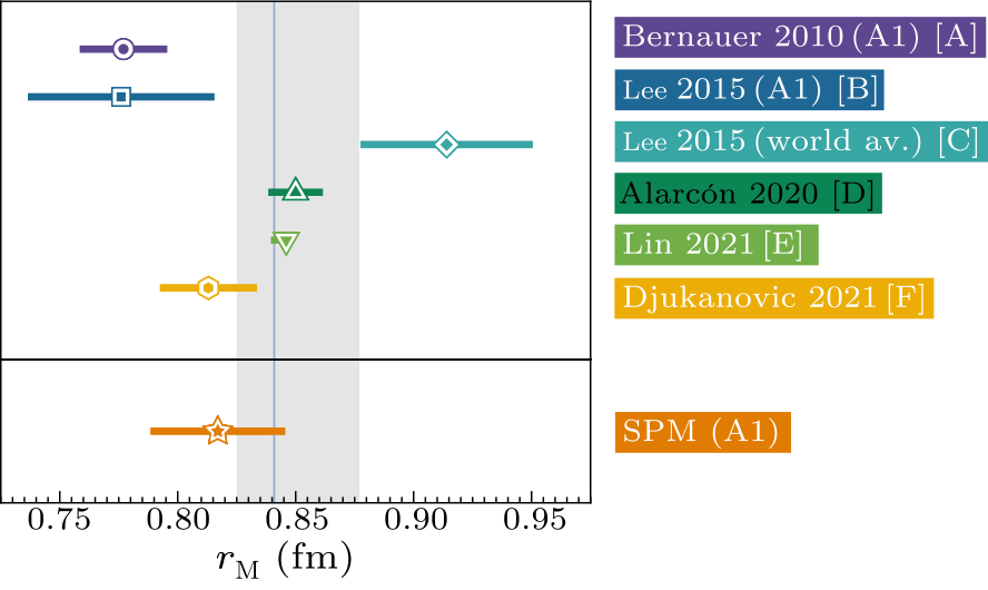
Fig. 1. Upper panel: Proton $r_{\scriptscriptstyle {\rm M}}$ extractions, obtained with various techniques: [A] = Refs. [27,28] (A1 Collaboration); [B] = Ref. [29] (A1 data); [C] = Ref. [29] (world average omitting A1 data); [D] = Ref. [30] (dispersion theory); [E] = Ref. [31] (dispersion theory); [F] = Ref. [32] (lattice quantum chromodynamics). The light-grey band is Eq. (6); within mutual uncertainties, this value agrees with $r_{\scriptscriptstyle {\rm E}}$ in Eq. (5), which is indicated by the thin vertical blue band. Lower panel: Result in Eq. (10), obtained from the data in Ref. [27] using the Schlessinger point method (SPM)[33–35] as described herein.
The proton radius controversy[36] demonstrated that a sound extraction of hadron radii from form factors measured in lepton+hadron scattering requires precise data, densely packed at very low $Q^2$. Furthermore, in the analysis of that data, great care should be taken to eliminate all systematic error intrinsic to the choice of data fitting function.[37–45] Recently, a scheme was developed to circumvent any need for a specific choice of fitting function in analyzing form factor data.[46,47] Introduced in Refs. [33,34] and now often described as the statistical SPM, it has been honed in hadron physics applications, especially those which require interpolation and reliable extrapolation, e.g., Refs. [48–54]. The SPM builds form-unbiased interpolations of data as the foundation for well constrained extrapolations. Herein, we employ it to extract $r_{\scriptscriptstyle {\rm M}}$ from the A1 data.[27,28] Before proceeding, it is worth remarking that the efficacy of the SPM rests firmly upon its mathematical connection with the Padé approximant. Indeed, the procedure might equally be called the multipoint Padé approximants technique. Owing to the properties of analytic functions, then with $N>0$ perfect values of such a function, ${\mathcal f}$, at discrete real points, ${\mathcal D}=\{x_i\,|\,i=1,\ldots,N\}$, the SPM will return an accurate representation of ${\mathcal f}(x)$ within a radius of convergence fixed by that one of the function's branch points which lies closest to the domain ${\mathcal D}$. A simple example is provided by a monopole: ${\mathcal f}(x)=1/(1+x)$, represented by $N$ points, each one lying on the curve, with $N$ large. Using any one of those points, the SPM will exactly reproduce ${\mathcal f}(x)$. To counter the problem that perfect function values are impossible to obtain, a powerful statistical aspect may be introduced. Namely, one chooses $M \lesssim N/2$ points at random from ${\mathcal D}$ and considers the associated function values. Using the SPM with each pair, $[x_i,{\mathcal f}(x_i)]$, one obtains a collection of analytic approximations to the monopole whose spread measures the uncertainty inherent in the numerical calculation. Each one of the approximations is of practically equal quality to the best least-squares fit to ${\mathcal f}$ as defined by the points in ${\mathcal D}$. There is no qualitative difference when extending these ideas to more sophisticated functions. Naturally, dealing with such “imperfections” is crucial when treating experimental data, as is the introduction of the smoothing procedure described below. 2. SPM and Proton Form Factor Data. The data obtained by the A1 Collaboration relate simultaneously to the proton electric and magnetic radii. They comprise $1400$ cross-sections measured with beam energies (in GeV): $0.18$, $0.315$, $0.45$, $0.585$, $0.72$, $0.855$. Focusing on the electric form factor, Ref. [46] worked with $N=40$ cross-section points in the low-$Q^2$ interval: $3.8 \times 10^{-3} \leq Q^2/{\rm GeV}^2 \leq 1.4\times10^{-2}$; and applied to this data, the SPM yielded: $$ r_{\scriptscriptstyle {\rm E}}^{\rm A1{\text{-}}SPM} = 0.856 \pm 0.014_{\rm stat}\,{\rm fm}.~~ \tag {7} $$ Since details are available in Ref. [46] hereafter we only sketch the SPM via its use in extracting $r_{\scriptscriptstyle {\rm M}}$. Regarding A1 data on the magnetic form factor, one finds in the Supplementary Material of Ref. [28] $77$ points describing a Rosenbluth separation[55] of the $ep$ cross-sections into results for $G_{\scriptscriptstyle {\rm E,M}}$ on the domain $1.5\times 10^{-2} \leq Q^2/{\rm GeV}^2 \leq 0.55$. The first nine $G_{\scriptscriptstyle {\rm M}}$ points are too noisy to be useful, only adding uncertainty to the SPM result without altering the central value; so herein we report an analysis of the $N=68 G_{\scriptscriptstyle {\rm M}}$ data on the domain ${\cal D}_{A1} = \{Q^2\,|\,2.7 \times 10^{-2} \leq Q^2/{\rm GeV}^2 \leq 0.55$}. In implementing the SPM, one constructs a prodigious number of continued fraction interpolations, every one encapsulating both local and global aspects of the curve underlying the data. The global quality is vital because it justifies use of the interpolations outside the domain of available data and thus enables and legitimizes evaluation of the curves' slope at the origin, i.e., use of Eq. (3). Of course, good data are statistically scattered around that curve which properly represents the form factor whose measurement is the aim; hence, they should not be directly interpolated. We address this issue by smoothing with a roughness penalty, following the procedure explained in Ref. [56] and made concrete in Section 3 of Ref. [46]. The approach is characterized by a well-defined optimal roughness penalty, $\epsilon$, whose value is a self-consistent output of the smoothing procedure: $\epsilon =0$ means that the data are untouched by smoothing whilst $\epsilon =1$ returns a linear least-squares realignment of the data. In the case of $r_{\scriptscriptstyle {\rm E}}$, considered in Ref. [46] and $r_{\scriptscriptstyle {\rm M}}$, herein, $\epsilon \simeq 0$. The ${\cal D}_{A1}$ set has $N=68$ points. From the data on ${\cal D}_{A1}$, we randomly select $L$ elements, with $7 \leq L \leq 19$. With a given value of $L$, one can generate $C(N,L)$ different interpolating functions, i.e., $O(9.7 \times 10^8 -3.3 \times 10^{15})$ interpolators. From the collection obtained using a given value of $L$, we select the first $5000$ that are smooth on the entire $Q^2$ domain covered by the data. Every interpolating function defines an extrapolation to $Q^2=0$, wherefrom $r_{\scriptscriptstyle {\rm M}}$ can be obtained via Eq. (3). So, for each value of $L$, $r_{\scriptscriptstyle {\rm M}}$ is determined by the average of all results computed from the $5000$ curves. To estimate the uncertainty in a particular SPM-determined value of $r_{\scriptscriptstyle {\rm M}}$, one must first reckon with the experimental error in the data. This is achieved herein by using a statistical bootstrap procedure.[57] We generate $1\,000$ copies of the set by replacing each element by a new point, distributed randomly about the mean defined by the element itself with variance equal to its associated error. Additionally, since $L$ is changed, there is a second error source $\sigma_{_{\scriptstyle \delta L}}$, which can be estimated by shifting $L\to L'$, repeating all steps for this new $L'$-value, and computing the standard deviation of the distribution of $r^{L}_{\scriptscriptstyle {\rm M}}$ for different $L$ values. Accordingly, one arrives at the SPM result: $r_{\scriptscriptstyle {\rm M}}\pm\sigma_r$; $$\begin{align} r_{\scriptscriptstyle {\rm M}}=\sum_{j=1}^{4}\frac{r^{{L_j}}_{\scriptscriptstyle {\rm M}}}{4};~~~\sigma_r=\Big[\sum_{j=1}^{4} \frac{(\sigma^{{L_j}}_r)^2}{4^2} +\sigma_{_{\scriptstyle \delta L}}^2\Big]^{1/2}.~~ \tag {8} \end{align} $$ For reasons explained below, we calculate results for each one of the values $L$ in ${\cal S}_L=\{L_j=3+4j\,\vert j = 1,2,3,4\}$. Thus, we have $20$-million results for $r_{\scriptscriptstyle {\rm M}}$, each computed from an independent interpolation. For all $j$ values in the range specified above, $\sigma_{_{\scriptstyle \delta L}}\ll \sigma_{r}^{ L_j}$; hence, the result is largely independent of the chosen value of $L$. 3. Validation of SPM Extrapolation on A1 Data. The keystone of any SPM data analysis is validation on the set. Herein, this means demonstrating that the radius returned by the SPM is reliable when used in connection with data on ${\cal D}_{A1}$. We accomplish this using the approach explained in the Supplementary Material of Ref. [46]. Step 1. The A1 Collaboration employed ten distinct data fitting models as the means by which to infer a result for $r_{\scriptscriptstyle {\rm M}}$.[28] From this collection, we selected the seven that are most straightforward to implement: (i) dipole; (ii) double dipole; (iii) polynomial; (iv) polynomial plus dipole; (v) polynomial times dipole; (vi) inverse polynomial; and (vii) Friedrich–Walcher parametrization.[58] Each of these models is connected with a distinct magnetic radius,[28] which defines the target input radius, $r_{\scriptscriptstyle {\rm M}}^{\rm input}$, that is, the SPM should recover (in fm): $r_{\scriptscriptstyle {\rm M}}^{\rm i} = 0.85$; $r_{\scriptscriptstyle {\rm M}}^{\rm ii} = 0.838761$; $r_{\scriptscriptstyle {\rm M}}^{\rm iii} = 0.779342$; $r_{\scriptscriptstyle {\rm M}}^{\rm iv} = 0.778892$; $r_{\scriptscriptstyle {\rm M}}^{v} = 0.775504$; $r_{\scriptscriptstyle {\rm M}}^{\rm vi} = 0.768562$; $r_{\scriptscriptstyle {\rm M}}^{\rm vii} = 0.807416$. Using every one of these models, we generated replicas of the A1 data built from the model values of $G_{\scriptscriptstyle {\rm M}}$ evaluated at the $Q^2$ points in ${\cal D}_{A1}$. The character of real data was modeled by scattering the values in response to fluctuations drawn according to a normal distribution. Step 2. Treating each of the seven sets as real, we determined the radius as described above. (I) Generate $10^3$ replicas. (II) Smooth each replica with the optimal parameter. (III) Use the SPM to obtain $r^{L_j}_{\scriptscriptstyle {\rm M}}$ and $\sigma^{L_j}_{\scriptscriptstyle {\rm M}}$, varying the number of input points $\{L_j=3+4j\,\vert j = 1,2,3,4\}$. (IV) Compute the final SPM result via Eq. (8) and compare it with the input value. The results of validation are summarized as follows: [A] For a given value of $L\in {\cal S}_L$ and all seven forms of fitting model, the distribution of SPM-extracted radii is a Gaussian, which is centered on the radius input value and whose characteristics are practically independent of $L$: in these cases, $\sigma_{_{\scriptstyle \delta L}}\ll \sigma^{{L_j}}_r$. We also considered $L \in {\cal O}_L=\{ M_{ji} = 3 + 4 j + i\,\vert\, j=1,2,3,i=1,2,3\}$. In these instances, however, one does not recover a satisfactory Gaussian distribution. So, we omit them from further consideration; to wit, we allow the validation process to impose a subset of $L$-values on our analysis, viz., $L\in {\cal S}_L$. [B] Defining the bias: $\delta r_{\scriptscriptstyle {\rm M}}=r_{\scriptscriptstyle {\rm M}}-r^{\rm input}_{\scriptscriptstyle {\rm M}}$, then the SPM extraction of the proton magnetic radius is robust: typically, $|\delta r_{\scriptscriptstyle {\rm M}}| \lesssim \sigma_r$, where $\sigma_r$ is the standard error in Eq. (8). The inverse polynomial model is the worst case. These remarks are illustrated in Fig. 2, which depicts $\delta r_{\scriptscriptstyle {\rm M}}$ as obtained using the SPM to recover $r_{\scriptscriptstyle {\rm M}}$ from each one of the seven $G_{\scriptscriptstyle {\rm M}}$ generators with their distinct $r_{\scriptscriptstyle {\rm M}}^{\rm input}$ values.
cpl-38-12-121401-fig2.png
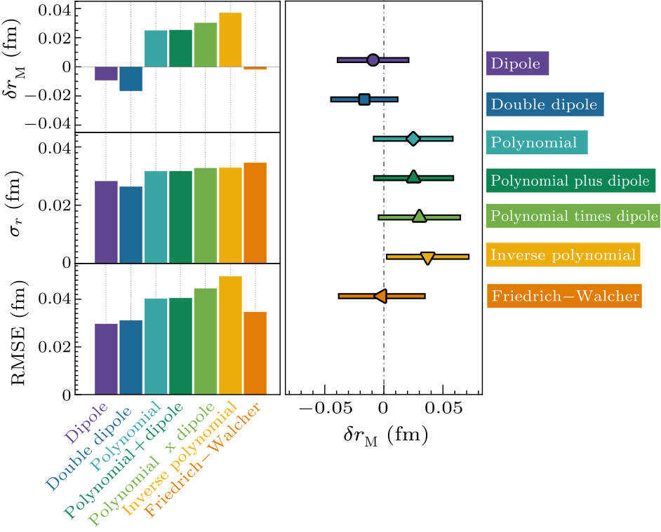
Fig. 2. Top and right panels: bias, $\delta r_{\scriptscriptstyle {\rm M}}=r_{\scriptscriptstyle {\rm M}}-r_{\scriptscriptstyle {\rm M}}^{\rm input}$, where the values of $r_{\scriptscriptstyle {\rm M}}^{\rm input}$ are listed in step 1. Middle panel: standard error, Eq. (8). Bottom panel: RMSE, Eq. (9), for SPM extractions of the proton magnetic radius from $5000$ replicas built using the seven models employed by the A1 Collaboration.[28]
[C] Considering the root-mean-square error: $$ \mathrm{RMSE}=\sqrt{(\delta r_{\scriptscriptstyle {\rm M}})^2+\sigma_r^2}\,,~~ \tag {9} $$ then, as revealed in Fig. 2, the SPM produces RMSE values which are approximatively independent of the model used to build the replicas. It therefore satisfies a standard “goodness-of-fit” criterion.[59] Hence, the SPM extraction of $r_{\scriptscriptstyle {\rm M}}$ may objectively be judged to return a reliable expression of the information contained in the data. 4. Proton Magnetic Radius from A1 Data. With the SPM now shown to return a reliable radius result from A1-like data, with its quoted errors, we turn to the real data on ${\cal D}_{A1}$ and obtain: $$ r_{\scriptscriptstyle {\rm M}}^{\rm A1{\text{-}}SPM} = 0.817 \pm 0.027_{\rm stat}.~~ \tag {10} $$ As evident in Fig. 1, within mutual uncertainties, this result agrees with that reported in Ref. [27], but the central value is 5.1% larger. This contrasts with our kindred extraction of $r_{\scriptscriptstyle {\rm E}}$ from A1 data, discussed elsewhere.[46] In that case, the central result from Eq. (7) is 2.6% lower. These differences have meaning in connection with Eq. (4). Writing $$ F_1^\prime(0) = {\mathcal d}_1 \frac{\mu_{\rm p}}{4 m_{\rm p}^2}, \; \frac{1}{\kappa_{\rm p}}F_2^\prime(0) = [{\mathcal d}_1-1-\delta_{_{\scriptstyle P}}] \frac{\mu_{\rm p}}{4 m_{\rm p}^2},~~ \tag {11} $$ then $b_{\scriptscriptstyle {\rm M}}^\perp>b_{\scriptscriptstyle {\rm E}}^\perp \; \forall \delta_{_{\scriptstyle P}}>-1$ and Eq. (4) is recovered with $\delta_{_{\scriptstyle P}}=0$. Working with the radii discussed above, the combinations of Eqs. (7) and (10), Eqs. (5) and (10), Eqs. (5) and (6) yield the results drawn in Fig. 3; namely: $$\begin{alignat}{1} \delta_{_{\scriptstyle P}}^{{\rm A1}_{\rm SPM}} &= \phantom{-}0.546 \pm 0.366,~~ \tag {12a}\\ \delta_{_{\scriptstyle P}}^{\rm {\rm A1}_{\rm SPM} + PDG} &= \phantom{-}0.329 \pm 0.321 ,~~ \tag {12b}\\ \delta_{_{\scriptstyle P}}^{\rm PDG } &= -0.147 \pm 0.322 ,~~ \tag {12c} \end{alignat} $$ of which the uncertainty-weighted average is $\delta_{_{\scriptstyle P}}=0.218 \pm 0.193$. Since the low-$Q^2$ behavior of $[1-\mu_{\rm p} G_{\scriptscriptstyle {\rm E}}(Q^2)/G_{\scriptscriptstyle {\rm M}}(Q^2)]$ is proportional to $\delta_{_{\scriptstyle P}}$, greater accuracy might be achieved through new high-precision low-$Q^2$ polarization-transfer measurements of $\mu_{\rm p} G_{\scriptscriptstyle {\rm E}}(Q^2)/G_{\scriptscriptstyle {\rm M}}(Q^2)$, as also remarked elsewhere.[19]
cpl-38-12-121401-fig3.png
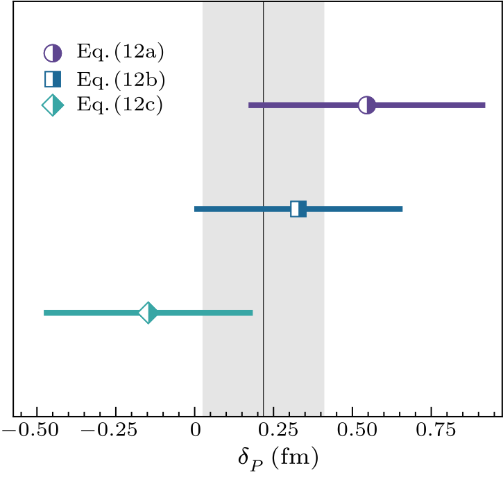
Fig. 3. Experiment-based results for deviations ($\delta_{_{\scriptstyle P}} \neq 0$) from Eq. (4) as listed in Eqs. (12). The vertical grey line together with the associated band show the uncertainty-weighted average.
5. Discussion and Conclusions. Figure 3 reveals that analyses of available data are consistent with Eq. (4) at a 26% confidence level. Namely, they suggest with this probability that the proton's Dirac and Pauli radii are not truly independent observables; instead, their difference is completely fixed by the proton Foldy term.[18] At worst, Eq. (4) is established as a useful approximation. Moreover, the analyses indicate with great certainty that the proton's Pauli radius is larger than its Dirac radius. These conclusions will serve as valuable constraints on pictures of proton structure. Their importance is elevated by the fact that any discussion of the “size” of the “absolutely” stable proton leads naturally to a discussion of confinement.[60,61] Namely, the empirical fact that the gluon and quark quanta associated with the fields used to define quantum chromodynamics (QCD), the strong interaction part of the Standard Model, have never been observed in a detector. Confinement has been linked with the phenomenon of emergent hadron mass (EHM),[62–64] viz., the appearance of nuclear-size masses for strong interaction systems comprised of massless field quanta. The QCD proton is just such a bound state: seeded by three light valence quarks, i.e., two $u$ quarks and one $d$ quark, which are all massless in the absence of Higgs boson couplings into QCD. Symmetries in quantum field theory entail that a massless fermion cannot possess an anomalous magnetic moment;[65–67] and, in the absence of any strong corrections, the anomalous magnetic moment of a light fermion is small. Yet, the proton's Pauli form factor, which expresses all its anomalous magnetic properties, is large on $Q^2\simeq 0$ and has a radius fixed (perhaps approximately) by Eq. (4). An explanation for the infrared scale of $F_2$-proton may be found in EHM:[62–64] realized most fundamentally in QCD via the dynamical generation of running masses for gluons, i.e., QCD's gauge bosons, and quarks;[68–70] and expressed in manifold corollaries.[70–72] For example, the running masses that owe to EHM are large at infrared momenta, with that of the quark being $\sim$$m_{\rm p}/3$, and the same phenomenon also endows dressed light quarks with anomalous magnetic moments that are $\sim$$\kappa_{\rm p}/3$ in the infrared. This explains the size of $F_2(0)$. Given then Eq. (4), even as an approximation, the amount by which the proton's light-front transverse mean-square magnetic radius exceeds the analogous charge radius is also seen to be (predominantly) determined by EHM. (Numerous theory analyses indicate that EHM also strongly influences $F_1(Q^2)$, with effects flowing into both the proton wave function and electromagnetic current via the running light quark masses.[8–11]) This discussion suggests that the scales underlying the proton's anomalous magnetization form factor may be attributed to EHM. Lacking, however, is quantitatively precise theory that can match QCD with Eqs. (4) and (12). There are many possible contributions to $F_2(Q^2\simeq 0)$, including:[7–11,73–78] quark anomalous magnetic moments, quark orbital angular momentum within the proton, meson cloud contributions to one or both, etc.; and related influences on $F_1(Q^2\simeq 0)$. An insightful understanding of the accuracy of Eq. (4) will demand an explanation of how all these factors might combine to produce a simple algebraic outcome; and, in step with that, experiments and associated analyses that deliver a precise result for $r_{\scriptscriptstyle {\rm M}}$ so that a veracious benchmark is provided. Acknowledgments. We are thankful for constructive comments from L. Chang, J. Friedrich, D. W. Higinbotham, R. J. Holt, V. Mokeev, W.-D. Nowak and J. Segovia. Use of the computer clusters at the Nanjing University Institute for Nonperturbative Physics is gratefully acknowledged.
References The Connection Between Spin and StatisticsNull-plane dynamics of particles and fieldsElectron Scattering and Nuclear StructureThe structure of the nucleon: Elastic electromagnetic form factorsExplanation and prediction of observables using continuum strong QCDBaryons as relativistic three-quark bound statesStrong QCD from Hadron Structure ExperimentsDiquark correlations in hadron physics: Origin, impact and evidenceHigh-Energy Behavior of Nucleon Electromagnetic Form FactorsTransverse Charge DensitiesTenth-Order QED Contribution to the Electron g 2 and an Improved Value of the Fine Structure ConstantComplete Tenth-Order QED Contribution to the Muon g 2 �ber die magnetische Ablenkung von Wasserstoffmolek�len und das magnetische Moment des Protons. I G E p / G M p Ratio by Polarization Transfer in e p e p Neutron-Electron InteractionProton Electromagnetic-Form-Factor Ratios at Low Q 2 The size of the protonProton Structure from the Measurement of 2S-2P Transition Frequencies of Muonic HydrogenThe Rydberg constant and proton size from atomic hydrogenA small proton charge radius from an electron–proton scattering experimentA measurement of the atomic hydrogen Lamb shift and the proton charge radiusTwo-photon frequency comb spectroscopy of atomic hydrogenLaser spectroscopy of muonic deuteriumHigh-Precision Determination of the Electric and Magnetic Form Factors of the ProtonElectric and magnetic form factors of the protonExtraction of the proton radius from electron-proton scattering dataPrecise determination of the proton magnetic radius from electron scattering dataDispersion-theoretical analysis of the electromagnetic form factors of the nucleon: Past, present and futureIsovector electromagnetic form factors of the nucleon from lattice QCD and the proton radius puzzleUse of Analyticity in the Calculation of Nonrelativistic Scattering AmplitudesAnalyticity as a Useful Computation ToolThreshold energies and poles for hadron physical problems by a model-independent universal algorithmThe proton charge radiusPolynomial fits and the proton radius puzzleReduction of the proton radius discrepancy by 3 σConsistency of electron scattering data with a small proton radiusProton radius from electron scattering dataEvaluation of low-Q2 fits to ep and ed elastic scattering dataReexamining the proton-radius problem using constrained Gaussian processesProton charge radius extraction from electron scattering data using dispersively improved chiral effective field theoryHow analytic choices can affect the extraction of electromagnetic form factors from elastic electron scattering cross section dataThe proton radius: from a puzzle to precisionFresh Extraction of the Proton Charge Radius from Electron ScatteringPion charge radius from pion+electron elastic scattering dataNucleon-to-Roper electromagnetic transition form factors at large Q 2 Distribution amplitudes of heavy-light mesonsSpectral functions of confined particlesScattering amplitudes and contour deformationsSemileptonic decays of D ( s ) mesonsSemileptonic B → η,J/ψ transitionsValence quark ratio in the protonHigh Energy Elastic Scattering of Electrons on ProtonsSmoothing by spline functionsA coherent interpretation of the form factors of the nucleon in terms of a pion cloud and constituent quarksRobust extraction of the proton charge radius from electron-proton scattering dataON THE IMPLICATIONS OF CONFINEMENTPion and kaon structure at the electron-ion colliderEmpirical Consequences of Emergent MassOn mass and matterAnomalous magnetic moment of light quarks and dynamical symmetry breakingAnomalous magnetic moment of quarksDressed-Quark Anomalous Magnetic MomentsThe gluon mass generation mechanism: A concise primerQCD at finite temperature and chemical potential from Dyson–Schwinger equationsInsights into the emergence of mass from studies of pion and kaon structureResolving the Bethe–Salpeter KernelRevealing the structure of light pseudoscalar mesons at the electron–ion colliderAnalysis of nucleon electromagnetic form factors from light-front holographic QCD: The spacelike regionElastic electromagnetic form factors of vector mesonsProton structure from a light-front HamiltonianNucleon elastic form factors at accessible large spacelike momentaVector-meson production and vector meson dominance
[1]Streater R F and Wightman A S 1980 PCT, Spin and Statistics and All That 3rd edn (New York: W. A. Benjamin, Inc.)
[2] Pauli W 1940 Phys. Rev. 58 716
[3]Weinberg S 2005 The Quantum Theory of Fields (Cambridge: Cambridge University Press) vol 1
[4] Coester F 1992 Prog. Part. Nucl. Phys. 29 1
[5]Zyla P et al. 2020 Review of Particle Physics, PTEP 2020 083C01
[6] Hofstadter R 1956 Rev. Mod. Phys. 28 214
[7] Punjabi V, Perdrisat C F, Jones M K, Brash E J, and Carlson C E 2015 Eur. Phys. J. A 51 79
[8] Cloet I C and Roberts C D 2014 Prog. Part. Nucl. Phys. 77 1
[9] Eichmann G, Sanchis-Alepuz H, Williams R, Alkofer R, and Fischer C S 2016 Prog. Part. Nucl. Phys. 91 1
[10] Brodsky S J et al. 2020 Int. J. Mod. Phys. E 29 2030006
[11] Barabanov M Y et al. 2021 Prog. Part. Nucl. Phys. 116 103835
[12] Sachs R 1962 Phys. Rev. 126 2256
[13] Miller G A 2010 Annu. Rev. Nucl. Part. Sci. 60 1
[14] Aoyama T, Hayakawa M, Kinoshita T, and Nio M 2012 Phys. Rev. Lett. 109 111807
[15] Aoyama T, Hayakawa M, Kinoshita T, and Nio M 2012 Phys. Rev. Lett. 109 111808
[16] Frisch R and Stern O 1933 Z. Phys. 85 4
[17] Jones M K et al. 2000 Phys. Rev. Lett. 84 1398
[18] Foldy L L 1958 Rev. Mod. Phys. 30 471
[19] Miller G A, Piasetzky E, and Ron G 2008 Phys. Rev. Lett. 101 082002
[20] Pohl R et al. 2010 Nature 466 213
[21] Antognini A et al. 2013 Science 339 417
[22] Beyer A et al. 2017 Science 358 79
[23] Xiong W et al. 2019 Nature 575 147
[24] Bezginov N, Valdez T, Horbatsch M, Marsman A, Vutha A C, and Hessels E A 2019 Science 365 1007
[25] Grinin A, Matveev A, Yost D C, Maisenbacher L, Wirthl V, Pohl R, Hänsch T W, Udem T 2020 Science 370 1061
[26] Pohl R et al. 2016 Science 353 669
[27] Bernauer J C et al. 2010 Phys. Rev. Lett. 105 242001
[28] Bernauer J C et al. 2014 Phys. Rev. C 90 015206
[29] Lee G, Arrington J R, and Hill R J 2015 Phys. Rev. D 92 013013
[30] Alarcón J M, Higinbotham D W, and Weiss C 2020 Phys. Rev. C 102 035203
[31] Lin Y H, Hammer H W, and Meißner U G 2021 Eur. Phys. J. A 57 255
[32] Djukanovic D, Harris T, von Hippel G, Junnarkar P M, Meyer H B, Mohler D, Ottnad K, Schulz T, Wilhelm J, and Wittig H 2021 Phys. Rev. D 103 094522
[33] Schlessinger L 1968 Phys. Rev. 167 1411
[34] Schlessinger L and Schwartz C 1966 Phys. Rev. Lett. 16 1173
[35] Tripolt R A, Haritan I, Wambach J, and Moiseyev N 2017 Phys. Lett. B 774 411
[36] Gao H and Vanderhaeghen M 2021 arXiv:2105.00571 [hep-ph]
[37] Kraus E, Mesick K E, White A, Gilman R, and Strauch S 2014 Phys. Rev. C 90 045206
[38] Lorenz I T and Meißner U G 2014 Phys. Lett. B 737 57
[39] Griffioen K, Carlson C, and Maddox S 2016 Phys. Rev. C 93 065207
[40] Higinbotham D W, Kabir A A, Lin V, Meekins D, Norum B, and Sawatzky B 2016 Phys. Rev. C 93 055207
[41] Hayward T B and Griffioen K A 2020 Nucl. Phys. A 999 121767
[42] Zhou S, Giulani P, Piekarewicz J, Bhattacharya A, and Pati D 2019 Phys. Rev. C 99 055202
[43] Alarcón J M, Higinbotham D W, Weiss C, and Ye Z 2019 Phys. Rev. C 99 044303
[44] Barcus S K, Higinbotham D W, and McClellan R E 2020 Phys. Rev. C 102 015205
[45] Hammer H W and Meißner U G 2020 Sci. Bull. 65 257
[46] Cui Z F, Binosi D, Roberts C D, and Schmidt S M 2021 Phys. Rev. Lett. 127 092001
[47] Cui Z F, Binosi D, Roberts C D, and Schmidt S M 2021 Phys. Lett. B 822 136631
[48] Chen C, Lu Y, Binosi D, Roberts C D, Rodrı́guez-Quintero J, and Segovia J 2019 Phys. Rev. D 99 034013
[49] Binosi D, Chang L, Ding M, Gao F, Papavassiliou J, and Roberts C D 2019 Phys. Lett. B 790 257
[50] Binosi D and Tripolt R A 2020 Phys. Lett. B 801 135171
[51] Eichmann G, Duarte P, Peña M P, and Stadler A 2019 Phys. Rev. D 100 094001
[52] Yao Z Q, Binosi D, Cui Z F, Roberts C D, Xu S S, and Zong H S 2020 Phys. Rev. D 102 014007
[53] Yao Z Q, Binosi D, Cui Z F, and Roberts C D 2021 Phys. Lett. B 818 136344
[54] Cui Z F, Gao F, Binosi D, Chang L, Roberts C D, and Schmidt S M 2021 arXiv:2108.11493 [hep-ph]
[55] Rosenbluth M 1950 Phys. Rev. 79 615
[56] Reinsch C H 1967 Numer. Math. 10 177
[57]Press W H, Teukolsky S A, Vetterling W T, and Flannery B P 2007 Numerical Recipes 3rd edn (New York: Cambridge University Press)
[58] Friedrich J and Walcher T 2003 Eur. Phys. J. A 17 607
[59] Yan X, Higinbotham D W, Dutta D, Gao H, Gasparian A, Khandaker M A, Liyanage N, Pasyuk E, Peng C, and Xiong W 2018 Phys. Rev. C 98 025204
[60] Roberts C D, Williams A G, and Krein G 1992 Int. J. Mod. Phys. A 7 5607
[61]Jaffe A M 2006 Not. Am. Math. Soc. 53 652
[62] Aguilar A C et al. 2019 Eur. Phys. J. A 55 190
[63] Roberts C D 2020 Symmetry 12 1468
[64] Roberts C D 2021 AAPPS Bull. 31 6
[65] Singh J 1985 Phys. Rev. D 31 1097
[66] Bicudo P J A, Ribeiro J E F T, Fernandes R 1999 Phys. Rev. C 59 1107
[67] Chang L, Liu Y X, and Roberts C D 2011 Phys. Rev. Lett. 106 072001
[68] Aguilar A C, Binosi D, and Papavassiliou J 2016 Front. Phys. Chin. 11 111203
[69] Fischer C S 2019 Prog. Part. Nucl. Phys. 105 1
[70] Roberts C D, Richards D G, Horn T, and Chang L 2021 Prog. Part. Nucl. Phys. 120 103883
[71] Qin S X and Roberts C D 2021 Chin. Phys. Lett. 38 071201
[72] Arrington J et al. 2021 J. Phys. G 48 075106
[73]Giannini M M and Santopinto E 2015 Chin. J. Phys. 53 020301
[74] Sufian R S, de Téramond G F, Brodsky S J, Deur A, and Dosch H G 2017 Phys. Rev. D 95 014011
[75] Xu Y Z, Binosi D, Cui Z F, Li B L, Roberts C D, Xu S S, and Zong H S 2019 Phys. Rev. D 100 114038
[76] Mondal C, Xu S, Lan J, Zhao X, Li Y, Chakrabarti D, and Vary J P 2020 Phys. Rev. D 102 016008
[77] Cui Z F, Chen C, Binosi D, de Soto F, Roberts C D, Rodríguez-Quintero J, Schmidt S M, and Segovia J 2020 Phys. Rev. D 102 014043
[78] Xu Y Z, Chen S, Yao Z Q, Binosi D, Cui Z F, and Roberts C D 2021 Eur. Phys. J. C 81 895